
This is the fifteenth “research” thread of the Polymath16 project to make progress on the Hadwiger–Nelson problem, continuing this post. This project is a follow-up to Aubrey de Grey’s breakthrough result that the chromatic number of the plane is at least 5. Discussion of the project of a non-research nature should continue in the Polymath proposal page. We will summarize progress on the Polymath wiki page.
At this point, much of the effort is transitioning to the writing stage, which is taking place on Overleaf. See this comment to obtain writing privileges for the paper. This thread can be used to discuss the write-up as well as any remaining research items.

Tom just posted something in the previous thread:
to which I say:
Wow, amazing! I can’t imagine how many months it would have taken me to code such a thing. This is so cool.
How hard do you think it would be to go from here to a systematic enumeration of the possible ways to improve on the diameter of Philip’s disk? (Plus, if you’re right, a similar enumeration of the 7-colour options for a sphere?)
I think the simulation is too slow for that kind of work. But, maybe I’ll try tiling a graph with SAT rules like Philip mentioned here: https://dustingmixon.wordpress.com/2018/06/24/polymath16-eighth-thread-more-upper-bounds/#comment-4934
The simulation will help determine if the SAT result is valid or if there’s a rule that needs to be added. Hopefully only simple rules are needed!
I’m not sure how to enumerate planar graphs, but maybe I’ll start by making Philip’s graph all triangles and allow the solver to remove edges.
I posted some updates here:
https://groups.google.com/forum/#!topic/hadwiger-nelson-problem/J_Tw1_hUxQI
For graphs with radius ~2 and above, the SAT-solver was providing solutions where complicated multi-tile constraints prevent the solution from actually working.
So, I tried a systematic enumeration, like you suggested. The simulator would decide if a graph was valid or not. The enumeration isn’t perfect, but works decently well. Also, it currently only generates graphs with triangles and quadrilaterals. The largest 6-color graph it found basically matches Gibbs’, but with some extra uninteresting garbage on the perimeter.
Wow, this is brilliant Tom. I’ll reply properly in a new post since this is quite high up the page.
I’m trying to dig into a probabilistic approach. So far, it turns out that for two forbidden distances, the chromatic number of the plane is at least 7. . The result is a graph with 8 vertices of degree 6 and 4 non-edges. If we allow 6-coloring, then 2 of 4 non-edges will turn out to be monochromatic with a total probability of less than 2, which leads to a contradiction. I’ll attach the picture a bit later.
I just added two vertices to the graph of Peter for
Maybe I’m doing something wrong?
The graph:
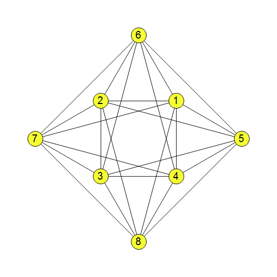
Nice, this indeed seems to prove that with these two forbidden distances CNP>=7. Repeating your argument slightly differently, in expectation strictly less than 2 of the 4 non-edges will be monochromatic, so sometimes 3 of them are bichromatic, thus we have a .
.
Yes. It’s brilliant. Bravo Jaan! I would say this is one of the most significant results of the whole project. I think it gives us a strong motivation to search for 2-distance graphs with even higher density, to see if we can push the CNP higher than 7.
Happy Christmas everybody!
Edge density, I of course meant.
This diamond has long been in the showcase, I just walked by and brushed the dust off of it. Thank you, but here I’m more skeptical so far.
First, I do not quite understand the probabilistic approach. Although, as I see from the comments, I’m moving in the right direction. Probability is one of those elusive things that behave in completely unpredictable ways.
For example, I still don’t feel the ground under my feet in Proposition 36. There are too many mono-non-mono inversions, and I get lost in them.
I have a lot of questions. Now I reduce them to the following.
How to move from a probabilistic approach to a specific graph in which you no longer need to operate with the concept of probability? How to estimate the minimum number of vertices of such a graph? , then the number of vertices can be roughly estimated as
  , where
  is the number of vertices of probabilistic graph, and
  , that is, for
  and
and  we get 1504 vertices. How optimistic is this estimate? How to construct an explicit graph?
My attempt. If for 6-coloring the probability
Also, for me, the essence of the concept of a chromatic number with two forbidden distances is not very clear. What do we do with this dragon? But in order not to dump everything in a heap, on this issue I’d better start a new chain.
I don’t think that we get any quantitative bound from the proof of Prop 36; even if we did, it should depend on the number of vertices of the graph used in the proof rather than on , although these are often correlated.
Ok, do you have any idea how to get the graph or to estimate its order?
No, in fact, as far as I know, theoretically it is even possible that the existence of such a graph depends on the axiom of choice…
So far, we have considered the lower bound for the chromatic number of a plane with two forbidden distances . We can go from the back and see how the upper bound behaves depending on the second distance
  (first distance is assumed to be 1, and also
  ). I hastily got some rough estimates using tiling the plane with regular hexagons with a diameter 1. Estimates can be improved. Please correct me, where I’m wrong. With increasing
  , the following picture is observed:
 we have
 we have
 we have
 , we have the proportional dependence
for
for
for
for large
If the latter is true, then one asks what gives us a chromatic number with two distances in general and its lower bound in particular? So far I do not see, for example, how it can be used to go closer to the chromatic number of a plane
  .
.
Thank you. Your argument is very clear.
By the way, maybe this bound can be improved, bearing in mind Pritikin or something like this.
Let . Then Pritikin will not help, and there is no way to reduce the upper bound
 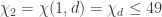 . Or what do you think?
Yes, the only way to get a better upper bound would be to find ‘siamese’ tilings, i.e., ones where some tiles of the same color are closer than 1. So far we could not find any interesting examples for this. But if we could, then maybe it would be possible to make all tiles of one color class in the coloring for small enough, and make the coloring for 1 such that none of these contain tiles of the
  color for 1.
BTW, I think it’s better to use the notation or something like that.
We kinda need both, don’t we? It seems we definitely need something to denote the supremum and infimum of over all d, and it shouldn’t have a d in it.
I don’t think we can prove much about the infimum, as if d is close to 1, then the upper bound of 7 holds, and most likely it’s the same as CNP. So when we write a general upper bound, we can write , just like we used to write
  without any trouble.
For all n from 4 to 8, we have examples of two-distance graphs in which there are only n-4 non-edges. If we could push this to larger even n, we would generalise Jaan’s discovery and further raise the lower bound on the two-distance CNP (so long as the non-edges are long enough to have a p_d less than 1/2). Right? – any other requirements of such a graph?
Yes, I have a similar question: what constructive elements are we allowed to use here? Say, can we use spindling? (This could give a decrease of one mono-edge.) Further, probably, it is not necessary to pay attention to all non-edges that are in the graph (otherwise, in my opinion, further progress, will be difficult). If so, then we need clear rules, which non-edges are required, and which are not.
For example, if we add a vertex to an 8-vertex graph, the number of non-edges increases so that the probability argument does not work, but it is obvious that the graph has not become weaker.
I have just remembered this paper that was highlighted during the fourth thread:
https://www.sciencedirect.com/science/article/pii/S019566980300218X
It contains a long list of 5-vertex graphs whose ten distances take only three values. A lot of them have one such distance represented by only one pair of vertices. It may be worth going through them for ideas for 10-vertex graphs with all but six distances taking one of only two values.
For a 10-vertex graph, we must have 39 edges, that is, the average vertex degree should be almost 8. I hardly believe that such a density can be realized. On the other hand, the upper bound of the chromatic number is 9…12 for the second distance 1.7…2. That is, we still have to go and go from bottom to top if we believe that the lower and upper bounds should finally coincide. By the way, this is one of my questions, and I will ask it in a new chain. Therefore, it seems to me that we should pay more attention to the classification of non-edges, and we should find the rules by which some non-edges can be ignored when summing probabilities. Then we will have a chance to move on.
Peter looked a lot at two-distance graphs in Chapter 2 of his thesis:
Click to access agoston_peter.pdf
But we only looked for two non-edges, if I recall correctly. He also has a couple of tables (not in the thesis) with the best bounds for the number of edges in unit-distance and two-distance graphs.
Related to this, there’s a metatopic I would like to discuss. I’ve encouraged him to write up his findings about the above bounds and submit it to a conference, since these bounds didn’t come up until now during the project. Also, in general, I think the main policy of polymath of not publishing results separately combined with the situation that the deadline of this project has been extended, but the progress made is quite slow (sometimes with months of break between), is really not ideal for a student…
Many thanks Domotor. It would be great to see those tables. As for publication, I agree, but I would also reiterate that the option of publication in Geombinatorics also exists – though as an outsider I do not know how it compares with conference proceedings volumes in terms of prestige in the mathematics community, but it is very rapid.
> not ideal for a student…
I would use your best judgement here. I agree it’s awkward.
How do we know that the upper and lower bounds of the chromatic number of the plane must ultimately coincide? In other words, is the chromatic number of the plane, determined on the basis of graphs, and the chromatic number, determined by tiling the plane, the same chromatic number? Implicitly assumed to be yes. How reliable is this fact?
I am not talking about the lower and upper bounds, but about the very concept of chromatic number. As far as I understand, it is defined, roughly speaking, in terms of graphs. Is a tile-based definition equivalent? Or is there no such definition, and is this just a way to find the upper bound?
Tilings are just a means to find an upper bound, these can be different from the actual chromatic number. Graphs are just a means of finding a lower bound, this is known to be sharp if one assumes the axiom of choice (which we usually do). See this part of the wiki for colorings that are restricted to be tiled-based, in which case better bounds are known: http://michaelnielsen.org/polymath1/index.php?title=Hadwiger-Nelson_problem#Tile-based_colourings_.28tilings.29
I understand your answer so (in my terms). No, we do not know whether the lower and upper bounds will coincide. And it does not depend on our computing capabilities. It is likely that there are some other hidden reasons of a fundamental nature that will not allow these bounds to coincide.
I would disagree with the second part. Most people conjecture that the bounds will coincide. Having larger computing capabilities would be a way to show that they are equal, but some other argument could also work, like bichromatic origin, or the probabilistic formulation, or this: https://mathoverflow.net/questions/338437/move-one-element-of-finite-set-out-from-a-in-plane
OK, we don’t know, but we beleive, right?
Yes, we don’t know, but believe that they should be equal.
I have a question about Geombinatorics. How can one download articles that are published there? I tried access through several university VPN, and sci-hub, but cannot get access to any article there. If true (which I doubt), then this is stronger protected than paywalled Elsevier journals. Thanks!
I had the same question when I started getting interested in this field. Short story: there has never been online access to the journal, but I have become good friends with Soifer and I was able to work with him and his assistant to get all the back issues scanned. They are still in the process of indexing everything, but very soon all back issues will be available for free at the journal site.
That sounds great, thank you for that effort!
It is an absolute goldmine. I felt it was the least I could do to thank Soifer for everything he has done in this field.
I don’t know if this is too late, but I collected links to the arXiv versions of all the articles in the special issue containing Aubrey’s paper here: https://thehighergeometer.wordpress.com/2018/07/19/special-issue-of-geombinatorics-on-recent-progress-on-the-chromatic-number-of-the-plane/
I said already that I do not understand prop.36. Recently, my misunderstanding has only intensified. Peter tried to give me an explanation, but to no avail. I want to make another attempt and ask a question here.
We managed to reduce the basic construction (where I have questions) to three (or four, or five) vertices. We take two isosceles triangles ABD and DBC with a common side BD, with sides AD=DC=1, BA=BD=BC=d, choose d>1 so that there are no questions about the lengths, so AC>1. We assume that the probability p_d of the event “a pair of vertices at a distance d has the same color” is strictly equal to 1/2. My question is: how does this lead to a contradiction (i.e. leads to p_d <1/2)?
As I understood from the explanations, the key argument here is the probability of coloring pairs of vertices at distances not equal to 1 or d. Simplified construction (where this argument is already used, and which I don’t understand) has only three vertices ABC. So, attention. If we follow the argument of prop.36, the following is stated: if the colors of the vertices A and B are different, then it follows that with probability 1 the colors of A and C are also different. But why?
Here is my counterexample (which for some reason does not work). Let's color B in blue, A and C in red. (Colors A and C are the same.) I don’t see that we are forbidden to do this, even if p_d=1/2.
I don’t immediately understand the construction you describe here, but I do understand the six-vertex construction given in the first of the three proofs in Prop 36. Can you please go through THAT construction step-by-step and highlight where you’re getting stuck?
OK, let me pre-empt you, because I think I see where you’re getting stuck. I think what you’re missing is the implication of the assumption that p_d is exactly 1/2. If it is, then every single one of the infinitely many triangles in the plane whose sides are (1,d,d) must be coloured in such a way that one of the sides of length d is mono. Why? Well, every pair of points in the plane that is at distance d is a side of the same number (four) of (1,d,d) triangles. Thus, it follows that if any such triangle were trichromatic, some other such triangle would need to be monochromatic, because otherwise, fewer than half of the infinite number (yes, sorry for this abuse of terminology) of point pairs in the plane that are at distance d would be monochromatic, which would contradict the assumption that p_d is exactly 1/2. And no such triangle can be monochromatic, because one of the edges has length 1.
Does that help?
Wait a little bit.
Let’s simplify the task and take an infinite number of triangles, that is, we continue the chain of triangles that you are talking about, in both directions to infinity.
We can color it in two colors in two ways, up to a permutation of colors. Now, if we look not at colors, but at mono and non-mono, it really turns out that mono appears more often. Am I on the right track?
Now allow 3 colors…
Close. Let’s orient your chain of triangles so that the sides with length 1 are horizontal. Then we have an infinite horizontal strip in which half the lines of length d go from upper left to lower right, and the other half go from lower left to upper right. Now, looking at mono and non-mono as you say, we have that if p_d is exactly 1/2 then either all the “upper left to lower right” set are mono and all the “lower left to upper right” set are bi, or vice versa. Note that I said nothing about how many colours are being used.
In the actual construction in Prop 36, the chain of triangles is not straight but wavy: there, half the lines of length d are vertical and half of them are sloping. But the same thing works: if p_d is exactly 1/2, either all the vertical lines are mono and all the sloping ones are bi, or vice versa.
Hey, but this proves that p_d> 1/2, and we need the other way around.
No, you just wrote it wrongly. In your chain of triangles, mono appears LESS often: it can’t appear more often, because that would give a mono triangle somewhere, i.e. a mono point pair at distance 1.
Here I counted edges of AC-type.
I immediately mean the wavy chain. Which edges are we looking at, which are lengths d or not d (and not 1)?
OK, let’s focus on the wavy chain. Let us work with a large d for the moment, say d=2. Then the vertices have four different y-coordinates, let’s call them p,q,r,s in increasing order. Each q-vertex and r-vertex has degree 5 and each p-vertex and s-vertex has degree 3. The edges of length 1 are those between p-vertices and q-vertices and those between r-vertices and s-vertices. The vertical edges of length d are those between p and r and between q and s. The sloping edges of length d are those between q and r. Then, if we assume p_d is exactly 1/2, we have just two cases: case 1 is when the vertical d-edges are mono and the sloping d-edges are bi, and case 2 is when the sloping d-edges are mono and the vertical d-edges are bi. Those are the only options, because any other colouring would give more bichromatic d-edges than mono ones, contradicting p_d=1/2.
So now, let’s go back to your first message. You said: “If we follow the argument of prop.36, the following is stated: if the colors of the vertices A and B are different, then it follows that with probability 1 the colors of A and C are also different. But why?” Simply because AB and AC are both sloping d-edges, hence the situation where A and B are different but A and C are the same is neither case 1 nor case 2, hence it cannot happen when p_d = 1/2.
No, you did not understand my notation. My sloping edges are AB and BC, and AC is a horizontal edge.
Sorry, I miswote that – I said “AB and AC are both sloping d-edges” but I meant to say “AB and BC are both sloping d-edges”. It’s our fault for changing the labelling from what is written in Prop 36! 🙂
So actually no, Prop 36 does NOT say that if A and B are different and p_d = 1/2 then A and C are also different.
That’s just the point that says. Can you access the e-mail now?
OK, yeah, Prop 36 does implicitly say that if A and B are different and p_d = 1/2 then A and C are also different. But the reason it says it is because of what I wrote in my most recent post.
Let’s take the wavy chain and 2-coloring.
The first coloring option: A=B=C=1, D=2, then repeat.
The second coloring option: A=C=1, B=D=2, and so on.
In both options we get 1:1 mono and non-mono lengths d (AB, BD, BC, CD* and so on) and all edges of AC-type are mono.
2-colouring gives things that aren’t true, yes (and that’s no surprise). But try it with three colours and you won’t find a problem. Remember that if you continue the chain you will get a vertex E such that BE = AC.
I thought I introduced the notation quite clearly. Have to draw a picture.
You explained it fine, it’s just that your {A,B,C,D} are equivalent to {B,A,D,C} in the text on the wiki. I’m just writing a new explanation.
So let me try again. I will use your notation.
Clearly if A and B are the same and B and C are also the same then A and C are the same. (That’s my case 2.) But if A and B are different and p_d = 1/2, then B and D are the same, so B and C are different. (That’s my case 1.) Now, as you say, in isolation this does not tell us whether A and C are the same. But the problem is that overall, at most half of the point pairs at distance AC can be the same (because AC is more than 1/2). This means that at least half of the wavy chains must be case 1. Moreover, if _any_ case-1 chains have _any_ AC pairs mono, there must be more chains of case 1 than case 2. But that cannot be true, because every point-pair at distance d is a sloping edge of two chains and a vertical edge of two other chains. Therefore we can conclude that in all chains of case 1, all AC-like pairs are indeed bichromatic.
Let’s slow down. We agreed that there is a wavy chain, including vertical (BD), horizontal (AC) and sloping (AB, BC) edges, and there are two coloring options if we use the terms mono and non-mono. I will nevertheless repeat my results for the 2-coloring of this chain to check: the vertical and sloping edges in both options of the 2-coloring have p_d = 1/2, and p_h=1, where h is the length of the edge AC.
Now the problem is that p_h is too big. And now we must consider the chains in which the role of d goes to h. Right?
No. First of all, it is to be expected that we will encounter contradictions if wetry to 2-colour anything. The bounds derived by the probabilistic method are with respect to a particular assumption of the chromatic number of the plane. That’s why the cases on the wiki in which the upper bound is less than the lower bound constitute proofs that CNP>4. The only simple case that is independent of any assumption about the CNP is that p_d is always at most 1/2 if d is more than 1/2. Second, this whole chain idea is a bad way to think about the issue, because there are two typesof edge of length h; it is better just to stich with the original four points. Third, no, we do not consider the case in which the role of d goes to h.
I’m composing a new, self-contained explanation of the part of Prop 36 that proves p_d is strictly less than 1/2, that I hope will be clearer. Give mea few minutes.
How is probability p_d defined? Is it possible to define it, starting with tiling the plane? Doubtfully.
I’m not sure what you mean by “tiling” there. The definition of p_d is the proportion of pairs of points at distance d that are the same colour in a particular colouring of the whole plane.
There is a problem, how to determine this proportion. To illustrate: you can move an edge on a plane so that the ends describe circles of different diameters.
And I meant that you can start by tiling the plane and clearly show that mono is less common than non-mono.
OK, try this. I will continue with your notation, rather than the one in Prop 36 on the wiki. I’ve just realised that the thing you’re really asking about is not Prop 36 at all, but the weaker Prop 35. Tell me exactly where (if at all) I lose you below.
———————–
The essence of the probabilistic approach (for present purposes, anyway) is that, for any number f that is more than 1/2, if there is a (finite) unit-distance graph G in which there is exactly one vertex pair {P,Q} at distance f, and if there is a way to k-colour G such that P and Q are the same colour, then that colouring of G can only be used for at most half of the (infinitely many) copies of G that can be drawn in the plane.
The particular graph G that we are studying here is the four-vertex unit-distance graph ABCD in which the only edges are AD and CD. So all we know so far is that D is coloured differently than either A or C. The distances BA, BD and BC are all d, and the distance AC is f.
Now, we are going to assume (and then derive a contradiction from) the hypothesis that p_d = 1/2. We know that if p_d = 1/2, every triangle in the plane with side lengths {1,d,d} has exactly two vertices the same colour.
So now, back to G. Under the assumption that p_d = 1/2, we have (up to colour transposition) only three possibilities for the colouring of G:
– case X: B and D are colour 1, and A and C are colour 2
– case Y: B and D are colour 1, A is colour 2, and C is colour 3
– case Z: A, B and C are colour 1, and D is colour 2
These are the only colourings in which both the {1,d,d} triangles, namely ABD and BCD, have exactly two vertices the same colour.
So now, we have that in cases X and Z, A and C are the same colour, while in case Y, A and C are different colours. Thus, since we are assuming that f is more than 1/2, we can say that at least half of the (infinitely many) copies of G that can be drawn in the plane must be coloured according to case Y. (Note that we’re not assuming here that p_f = 1/2, only that it is at most 1/2.)
So this means that at most half of those copies of G are coloured according to case Z.
But wait: the probability that AB is mono is exactly 1/2 (because it is of length d), and Z is the only case where AB is mono. So in fact, at LEAST half the copies of G are case Z. And that means there is no space left for case X – in other words, in any copy of G for which A and B are different colours, A and C are also different colours. The contradiction follows by the logic of Prop 35, which I think you’re OK with (yes?).
Thanks, Aubrey. Yes, I want to limit our consideration to proving that the probability of a mono-pair is strictly less than half. No, I did not consider prop. 35.
And I will stop you at the very beginning. First of all, it is necessary to give an exact definition for probability p_d, and how it can be calculated. If such definition is given on the wiki, then I don’t understand it. I think this is my main difficulty.
All good. My first thought was to refer you back to Terry’s original post:
which sets this all out. However, on re-reading it, even though I’m sure it is very clear to professional mathematicians, I have a feeling that you will be no more familiar than I with concepts such as Haar measure, the Euclidean isometry group and finite versus countable additivity. Therefore, let me give my own definition. Fix a number k, and colour the entire plane randomly so that each point in the plane is assigned one of k colours but no pair of points at distance 1 are assigned the same colour. Then pick a point P at randon, and a second point Q on the circle with centre P and radius d. Record whether P and Q are the same colour. Then do it all again (the random colouring and the picking of P and Q). And again, a lot. Then p_d (with respect to k) is the limit, as we do this more and more times, of the proportion of cases in which P and Q were the same colour.
Does the term random coloring refer to a method of coloring, or only to movements of a plane already colored once and color permutations? (What is deterministic in Terry’s terminology?) In other words, can we color a plane once, and then randomly permute colors and select pairs of points P and Q? If not, why? What are the problems?
I don’t think it matters, but the situation is clearer if we recolour the plane each time.
OK. It matters to me, but we will drop these questions if you are in doubt.
Now I’m interested in the relationship of plane coloring with graphs, for example your (our) 4-vertex graph. I don’t see it yet. A graph cannot color the entire plane, no matter how many times you move it and how many times you check pairs.
I will explain. You defined p_d in terms of coloring the entire plane, but in the proof it is applied to graph coloring. I do not see how to move from one to another. Is there no way to define p_d in terms of graph coloring?
No, there isn’t. What graphs can do is provide bounds (upper and lower) on p_d, that’s all. (Just as they can only providelower bounds on the CNP.)
Then this is a transfer of the concept from one area of definition to another (significantly different), which in my opinion is wrong.
Just to illustrate. You claim that for each non-edge of length d, you can choose other non-edge such that we get a triangle with sides {1, d, d}. I agree with this, but I additionally affirm that for the same non-edge one can choose an infinite number of other non-edges forming triangles with sides {x>1, d, d}. Since the latter are clearly more, the contribution to the overall probability of the former is insignificant.
That doesn’t matter. The probability p_d is just the probability that two (randomly chosen) points at distance d will be the same colout. No triangles are involved in the definition of p_d. The utility of the {1,d,d} triangles arises only because they cannot be monochnomatic, which is what allows us to say that if p_d = 1/2 then they mustall be bichromatic and never trichromatic.
But I think, this does not say anything. If the probability p_d = 1/2 or even 3/4, then triangles can be any, for example all trichromatic. Because they are beaten by all the other triangles with base x.
No. Consider a (x,d,d) triangle and a {1,d,d} triangle that share two vertices. If the {x,d,d} triangle is monochromatic, the {1,d,d} one cannot be trichromatic. You can’t count the point pairs once for each triangle they are in – the point pair is either mono or it isn’t.
That doesn’t mean anything either. Let {1, d, d} be trichromatic and all triangles {x, d, d} bichromatic. This is enough to have more mono-non-edges than non-mono.
What? No it isn’t! In that scenario, even if you do count point-pairs twice (once for each shape of triangle), there are no mono d-edges in the {1, d, d} triangles and there are the same number of mono and bi d-edges in the {x, d, d} triangles, so for sure there are more non-mono d-edges than mono.
Let’s count. (Of course, we consider only non-edges of length d.)
Go on… Which of thoe d-edges are mono and which are bi?
Well, it is very difficult to understand from the drawing. Probably the two d-non-edges that are colored 1-2 and 1-3 are bichromatic non-edges, and the three ones that are colored 1-1 are mono. And how do you think?
That’s not good enough, because there are {1,d,d} triangles that you haven’t drawn – ones that have a 1-1 ege from your picture as one of their edges.
Well, imagine I drawn these triangles. But what does that change? In the triangles you are talking about, the lower side 1-1 is a non-edge, that is, it does not prohibit this side from being mono. The only edge with an unit distance in my picture is colored 2-3.
I’ll said it again. In my picture there is only one triangle {1, d, d} colored {1, 2, 3}. The rest ones are {x_i, d, d} with non-unit-distance x_i.
Or do you mean that I have to add new vertices to my picture so that new {1, d, d} triangles form? Then I do not understand why I should do this? That is, what is the logic of the formation of this graph? Is it possible to explicitly describe it as a set of rules?
The question we’re trying to address is whether more than half of the lines of length d can be mono. My answer is: no they can’t, because every such line is an edge of a {1,d,d} triangle, which has two such lines as edges, at least one of which is bi. I still don’t see why you think that this simple argument is in any way altered by considering {x,d,d} triangles. If you insist on considering {x,d,d} triangles, then consider one x at a time, and make chains of triangles in which the triangles alternate between {1,d,d} and {x,d,d}.
Hmm. And I still can’t understand why I should consider the triangles {1, d, d}? Well, actually, each non-edge of length d is the side of four triangles {1, d, d}. Why do we remember only one? What are the rules of the game? How does this simple argument that you are talking about relate to your definition of probability p_d?
We don’t remember only one, we remember all four – the only point that matters is that is that all such lines are associated with the same number of triangles, not what that number is. This argument does NOT relate to my DEFINITION of p_d, only to the simplest upper bound on the VALUE of p_d.
Good. It seems I’m starting to understand what is the matter. And I will try to explain why your simple argument from my point of view does not work. (Or in any case, it does not work in such an obvious way.)
So, we have reduced the original version of the problem and now it looks like this. We take the Euclidean plane, a certain number of colors k, necessary for its regular coloring (with forbidden distance 1), and choose a certain distance d (let d>1). Now, in some way, we scatter colored pairs of points on this plane, and in each pair the distance between the points is d. Pairs with other distances do not interest us yet. Next, we ask ourselves, can the number of mono-pairs exceed the number of non-mono-pairs?
To find the upper bound for fraction of mono-pairs, we fix some (non-random) set of pairs and try to color them so that the fraction of mono-pairs is maximal. Now the question is what kind of set of pairs it is, and what properties should it have in order to adequately describe the properties of the entire plane?
You want to convince me that the fraction of mono-pairs cannot be more than half of the total number of pairs. I don’t feel that you convinced me. The reason for my doubts is that (in my opinion) you offer too special set of pairs, and I see no reason why it should be just that, and not different.
Your simple argument: for each mono pair, you can pick up another pair, which will be non-mono. My counterargument: for each non-mono pair, you can choose several (let for definiteness, two) other mono pairs. We can play a game. Let’s say I start and draw a mono-pair. Your move, you add a non-mono-pair to it. My move, I double the number of mono pairs. Your move, you restore the status quo. Etc. After each of your moves, we will have a score of p_d = 1/2 (well, either less or equal, if you want), after each mine there will be p_d = 2/3. And I see no reason why we should stop after your move. Therefore, your argument does not convince me.
Now I will give a construction that can convince me, but still leaves questions. Take the original mono-pair. Now, instead of constructing a single triangle, you fix one of the vertices of this mono-pair and construct a circle of radius d. On this circle lies a side with unit length of infinite set of triangles.
Now, on the one hand, I will not be able to color more than half the circumference in the same color as the color of the center, and on the other, it will be difficult for me to find fault with the fact that we took some too special triangles, since we will take everything at once ( from some special class, though). Then you can fix the second vertex and do the same. And additionally you can draw circles of radius 1 to really cover all triangles of the form {1, d, d} with a given vertex.
By the way, if I’m not mistaken, such a construction for some d (for which the length of circumference is close to an odd integer) gives better estimates of the upper bound p_d.
Works for me. But you said “but still leaves questions” but then you didn’t ask any. What are the questions you were referring to?
The main question, as in the case of {1, d, d}-triangles: to prove that the construction used is adequate to the entire plane. The concept of p_d is defined for a plane, and we use it for a (incommensurably) small part of this plane. You implicitly assume such adequacy. And in my opinion, it requires proof.
We need to make sure that the circle-based approach works as expected, because I showed only the first step. In the second step, each pair of an infinite set of newly formed pairs (both mono and non-mono) is taken, and the same thing is done with it. That is, after two steps, we already get the “tiling” by triangles of part of the plane. The question will arise with what weighting factors these triangles should be taken into account (since the density of use of points will be different for the central and peripheral regions). Or we might think about how to adjust the circle-based approach so that this issue is resolved automatically.
The next question is how to adapt (in new terms) the proof that p_d is strictly less than half.
Such an adaptation may not be necessary for all d that do not form a regular polygon with an even number of vertices. This is if the circle-based approach really works.
You don’t need to worry about a weighting factor, because if you continue the process with an infinite number of steps then the process converges to uniform density. As for the strict inequality I don’t think you can use this for everything except even plygons – I think it only works for odd polygons, i.e. not for irrational fractions of pi. The constructions in Prop 35 and 36 are the way to go.
Looks like we’re back to where we started. I guess we did everything we could. Thank you.
Right folks, Tom has made what seems to me to be big progress on tilings. His post is a long way up the page:
so I’ll reply here.
Tom – I feel that this is already significant enough that we should find some way to include it in the paper, but I also get the sense that you can fairly straightforwardly push it further, albeit maybe not quite to the point of constituting a provably exhaustive search.
I’m not seeing your “vertices 0,1,2 above” – the labels aren’t showing up. Can you post the images here? We have a dropbox for that; alternatively just email them to me at aubrey@sens.org and I’ll do it.
Now I’ll have a look at your 5-colouring. It is certainly a close contender…
OK, for sure your 5-colouring is a new record. Amazing! (Well, after Bock’s discovery of a record-breaking strip, maybe I should not be so amazed.) Bravo!
The optimal way of drawing it, I think, is to have one 5-colour vertex. We start from the “previous best” (let’s use your version of it), and leave the vicinity of the bottom vertex of the red tile alone, but then we draw a line up from the midpoint of the top edge of the red tile., i.e. up the centre of the top blue tile. This lets us eliminate the lines that form the left and right edges of that blue tile and just have two tiles at the top, coloured blue and purple (ot sure whether it matters which way round) – all we need to do to make that work is to recolour the top-right purple tile yellow. Then it’s just a question of how far out the non-red tiles can be extended – possibly with the addition of small new tiles at the extremities.
Who can optimise this to an exact solution? I am too busy today, I’m afraid.
Ah, now I’m not so sure – your depiction of the previous best is somewhat truncated – see here for the true best:
https://drive.google.com/file/d/1-LEV4uzd2FjGBvC6cPUL0EDY2cjQy1FB/view
But you may still beat that… grrr I am so annoyed that I have day-job duties right now…
Here’s a rough sketch of what I was saying above. I think it slightly beats the previous record, but I’m not sure. Anyone?
Oh, yeah, I did truncate the previous best. Here’s another diagram with rigid edges included, if that helps.
I can’t tell if it’s actually better or not.
Thanks Tom. Looks to me as though the lower part is amenable to a little expansion – shouldn’t the circle pass through the yellow/orange point at 8 o’clock and the green/purple point at 4 o’clock? Maybe before that the very bottom tiles (green and orange) will become constraned, but they are a long way from that in your picture.
I think I’m almost seeing a diagram that could lead to an exact radius – not quite though 🙂
Hmm, yeah, there was nothing in my simulation to encourage a maximum radius. But, it was easy to make the simulation push the perimeter vertices away at a given radius. By gradually adjusting this radius, the vertices appear to settle optimally.
Great. I’m doing the algebra now and I’m agreeing accurately with your result for the previous record but I’m getting 1.21985 for the new construction. I may have an error – more soon – but either way it looks like we indeed have a new record. Yay!
And I did have an error, but I’m pretty sure I have it right now and my value is 1.21442. I’m still trying to remember how to get Mathematica to give me an exact expression as a root of a polynomial – maybe tomorrow 🙂
Hmm, when I try a radius .001 too big, I see that the these dotted lines are too long. So, I think they must be unit length. The simulation is very insistent that the maximum radius is 1.158, but maybe I goofed something up.
Gah, totally my bad – finally found my error and now I indeed get 1.15809. I’ll do the algebra tomorrow to get the exact expressions.
Bravo again Tom – that’s some seriously impressive code you’ve written. Very glad it has delivered some numerical progress!
re: “vertices 0,1,2 above”
The labels are there, but kind of faint. Clicking the image should show it in full size, which probably helps. Anyways, in those diagrams, vertex 0 corresponds to the central red tile. Vertices 1 and 2 are the adjacent blue and yellow tiles.
OK, just to conclude the analysis of Tom’s awesome 5-disc (and if I get the latex right it will be a total miracle):
The 5-disc we already knew about has a radius that is numerically about 1.090961732, being plus a root of
  .
.
The new 5-disc has a radius that is numerically about 1.158086135, being most economically described (according to Mathematica) in two steps. The distance x from the five-tile point to the edge of the disc, i.e. the length of the green/orange boundary at the bottom of Tom’s most recent picture, is numerically about 0.4813633443, being a root of . Then the radius of the disc is 1/18 of
  .
.
If someone else could check the above independently, e.g. with Maple, that would be great.
Whew, almost right. There should be a minus sign between “x” and “32” near the end of the last formula.
I added a few snippets to the table on discs and strips at the wiki. I think it is complete now other than that I forget where we are with the smallest disc covering a 5-chromatic graph – can someone remind me?
Ah, wait, I may have become confused. Jaan – here, when you get to 1.25:
you were referring to the diameter of a disc that contains a 4-chromatic graph, yes? I can’t find (well, I can’t convince myself that I have found) your best result for the strip that contains a 5-chromatic graph – is it 1.4 ?
Here’s a question that I don’t think anyone has yet addressed (in the project or in the literature), and which seems pretty natural:
What is the smallest area of a convex shape that cannot be k-coloured?
The upper bound will presumably be refined by finding (k+1)-chromatic graphs that fit inside increasingly small convex shapes, and the lower bound by finding the minimal area to truncate from that shape that renders it k-tileable while still convex. As such, the area (i.e. both bounds) is 0 for k=2, but I think it’s non-trivial even for k=3 (best upper bound I have so far is 1.63). What about higher k? Any other thoughts?
OK we can rather clearly do pi/2 🙂
You can do arbitrarily large area with three colors by taking a sufficiently thin, very long strip, no?
Sure. The question is how SMALL a convex shape we can find that is NOT k-colourable. Clearly we can take the convex hull of any (k+1)-chromatic graph as the upper bound. The question thus comes down to (a) finding (k+1)-chromatic graphs with small area, and then (b) finding ways to shave bits off such a graph’s convex hull to leave a convex shape that is still not k-tileable.
Oh, I see! Well, once we looked at the smallest possible rectangles, that’s all I know: https://dustingmixon.wordpress.com/2018/09/14/polymath16-eleventh-thread-chromatic-numbers-of-planar-sets/#comment-5696
Hi everyone – change of topic – back to higher-dimensional UDGs. I have a new construction that generalises my small graph in R^3, and for which the chromatic number for R^(2n-1) is 3n. This is of course weaker than the known exponential lower bound, and indeed it doesn’t even break any records for small n, but I think it is still noteworthy just because (AFAIK) it’s the first explicit construction that extends to arbitrarily high dimensions and does better than the value of n+2 for R^n achieved by the obvious spindle: if I’m not mistaken, none of the the brilliant constructions that hold the records for specific n are generalisable. The bad news is… I’m not 100% sure that my construction is actually embeddable 🙂 However, the better news is that it may be not just embeddable but extendable in a manner that achieves more, maybe even 2n for R^n, which at least would give a new record for R^5. (More on that below.) At any rate, this idea has now very much reached the Polymath zone, in that I’ve taken it far enough that I think I can explain it, but I’ve also reached the limit of what I feel able to do myself.
OK here goes. First I recall the construction for R^3, but I break it down with better notation than before.
———————————————–
1) We begin by taking a unit tetrahedron and pasting two more tetrahedra onto it. Call this six-vertex thing A. It has two vertices that are shared by all three tetrahedra, two that belong to only one tetrahedron, and two that belong to two. Call these the I-vertices, the P-vertices and the T-vertices respectively (these stand for “internal”, “pole” and “tropic”).
2) We then take two copies of A and identify both their P-vertices. This creates a ten-vertex structure that is not rigid: specifically, we can rotate the copies of A relative to each other so as to place the T-vertices attached to a given P-vertex at unit distance from each other. In this configuration, the four T-vertices form a square.
3) We then select a P-vertex, call it P_1, and attach a new vertex, which we denote F (“flap”), to the two T-vertices (one from each copy of A) that are NOT attached to P_1. (Here and hereafter, for avoidance of doubt, “attaching” means placing at unit distance and joining with an edge.) In other words, F is attached to the two T-vertices that are attached to the other P-vertex, P_2. We now have an 11-vertex structure that we call B. Note that F can be placed anywhere in a circle centred on the midpoint of the edge joining the two T-vertices to which it is attached.
4) We now take two copies of B, call them B_x and B_y. We identify P_1 of each – call this common vertex P_1 still – and we attach P_2_x to P_2_y. Now, both B_x and B_y can still rotate around their respective axes (lines between poles). This means we can place F_x and F_y at the same distance from P_1 and then rotate B_x and B_y to coincide the F’s as a single vertex F. Call this 20-vertex structure C (for “clamp”). Note, critically, that we have still not made the structure rigid: in particular, we have not committed to a particular distance between P_1 and F (though it must be between about 1 and 2.5).
5) Finally we take a “scaffold” structure S, with six vertices and lots of edges; it will be most convenient to use the unit-edge octahedron. For each pair of vertices of S that are not unit distance apart (of which there are just three, each being Sqrt[2] apart), we take a copy of C and identify its P_1 with one of the pair and its F with the other. Call this final structure D.
6) Now we check the chromatic number. Suppose we can colour C with five colours. Since P_2_x and P_2_y are attached, without loss of generality we can assume that P_2_x is a different colour than P_1; let us say P_1 is colour 1 and P_2_x is colour 2. Then the I-vertices of one of the two copies of A within B_x, call it A_x_v, can be assigned colours 3 and 4. Now consider the T-vertices of B_x; in particular, consider the pair T_x_1v and T_x_2v that are vertices of A_x_v. They are attached to P_1 and P_2_x respectively and also to each other. The only colourings that are available for them thus involve making T_x_2v colour 1 or making T_x_1v colour 2 (or both), since there is only colour 5 left. But wait: the same applies to the other two T-vertices, T_x_1w and T_x_2w (regardless of whether there is a different choice of colours for the I-vertices), and of course T_x_2v is also attached to T_x_2w. Thus, all the ways to colour the square of T-vertices end up with one or other of T_x_2v and T_x_2w being coloured 1. And that means F cannot be coloured 1 (since it is attached to both of them). But P_1 is coloured 1, so F and P_1 are different colours. And because the distance between P_1 and F can be chosen to be Sqrt[2], we can do step 5 of the construction and thus ensure that all six vertices of S must be different colours. Thus, either some copy of C needs six colours (which would allow its F and P_1 to be the same colour), or else S does – which, in combination, means that D does.
———————————————–
So now for the generalisation. I will describe it only for odd dimensions, where the analogy with R^3 is cleanest. We will work in R^(2n-1) and obtain a graph with chromatic number 3n.
———————————————–
1) We begin by taking a unit (2n)-simplex and pasting n more (2n)-simplices onto it. Call this (3n)-vertex thing A. It has n vertices that are shared by all n+1 simplices, n that belong to only one simplex, and n that belong to all but one. Call these the I-vertices, the P-vertices and the T-vertices respectively (these stand for “internal”, “pole” and “tropics”).
2) We then take n copies of A and identify all their P-vertices. This creates a (2n^2+n)-vertex structure that is not rigid: specifically, we can rotate the copies of A relative to each other so as to place the T-vertices attached to a given P-vertex unit distance from each other. In this configuration, the n^2 T-vertices form a graph that is the cross-product of two n-simplices.
3) We then select a P-vertex, call it P_1, and attach a new vertex, which we denote F (“flap”), to all the n T-vertices (one from each copy of A) that are NOT attached to P_1. We now have a (2n^2+n+1)-vertex structure that we call B. Note that F can be placed anywhere on the surface of a sphere centred on the midpoint of the simplex whose vertices are the T-vertices to which it is attached.
4) We now take n! (yes, factorial) copies of B. We identify one pole of each – call this common vertex P_1. Then we divide the copies of B into two equal-sized sets and identify the P_2’s within the sets, and attach the two P_2’s. Then we create a triangle P_3_1, P_3_2 and P_3_3 and distribute the P_3’s evenly, etc. In this way we straightforwardly ensure that, in any colouring, there is at least one copy of B that uses different colours for each of its P-vertices. Now, (I think!) the B’s can still “rotate”. This means (I think!) that we can place all the F’s at the same distance from P_1 and rotate the B’s to coincide the F’s as a single vertex F. Call this n!*n*(2n)+(n+1)C2+1-vertex structure C (for “clamp”). Note, critically, that (I think!) we have still not made the structure rigid: in particular, we have not committed to a particular distance between P_1 and F.
5) Finally we take a “scaffold” structure S, with at least 3n vertices and lots of edges; it will be most convenient to use the unit-edge octahedron-equivalent (is there a name for this, like hyperoctahedron?) in R^(2n-1), which has 4n-2 vertices. For n+1 of the pairs of vertices of S that are not unit distance apart (of which there are 2n-1 in total, each being Sqrt[2] apart), we take a copy of C and identify its P_1 with one of the pair and its F with the other. Discard the vertices of S to which we did not attach a copy of C. Call this final structure D; it has (n!*n*(2n)+(n+1)C2+1)*(n+1) vertices.
6) Now we check the chromatic number. Suppose we can colour C with 3n-1 colours. As noted above, without loss of generality we can choose x among the n! copies of B such that all its P-vertices are different colours; let us say P_i_x is colour i for i in 1..n. Then the I-vertices of one of the n copies of A within B_x, call it A_x_v, can be assigned colours n+1 through 2n. Now consider the T-vertices of B_x; in particular, consider the set T_x_i_v that are vertices of A_x_v. They are attached to their corresponding P_i_x and also to each other. The only colourings that are available for them thus involve making at least one of the T-vertices the (single) available colour in 1..n, since there are only n-1 colours left (namely 2n+1 though 3n-1). But wait: we chose v (i.e. our copy of A within B_x) arbitrarily, so the same applies to the n-1 other sets of T-vertices, T_x_i_w etc (regardless of whether there is a different choice of colours for the I-vertices), and of course T_x_i_v is also attached to T_x_i_w for any fixed i. Thus, all the ways to colour the n-simplex X n-simplex of T-vertices within C end up with (exactly) one of the T_x_1_v (v in 1..n) being coloured 1. And that means F cannot be coloured 1 (since it is attached to all of them). But P_1 is coloured 1, so F and P_1 are different colours. And because the distance between P_1 and F can (I think!) be chosen to be Sqrt[2], we can do step 5 of the construction and thus ensure that at least 3n vertices of S must be different colours. Thus, either some copy of C needs 3n colours (which would allow its F and P_1 to be the same colour), or else S does – which, in combination, means that D does.
———————————————–
Whew. OK, so as you can see I have not fully convinced myself that the necessary degrees of freedom exist. Steps 1 and 3 are unassailable; step 5 relies only on the ability to place F and P_1 at distance Sqrt[2], and I’m 99% sure that’s fine; and step 2 seems 99% certain to be OK too. It’s step 4 that I’m most hesitant about, because there are so many copies of B… but I think, by analogy with the R^3 construction, that the only degrees of freedom that we lose there are one rotational one for each copy of B, with no additional constraints on the distance of F from P_1.
And that’s what leads me to the hope that maybe we can get a scrap further, and in particular get to 10 for R^5 (i.e. n=3). Thing is, as noted at the end of step 3, the individual F’s that are attached to the copies of B are only attached to n T-vertices, so initially they each have not just one but n-1 degrees of freedom. If they indeed retain those degrees through step 4 (the merge of the F’s), then we can surely attach more than one F for a given set of rotations of the B’s, and of course that would mean we can arrange for the multiple F’s to form a simplex, which just MIGHT allow a way to squeeze the CN higher.
Well, I hope I’ve explained all this well enough for at least some of you to get the idea. Please shout if not!
Teeny correction to step 5: actually we can only discard one of each pair of vertices in the hyperoctahedron to which we did not clamp a copy of C. Thus the order of these graphs is actually (2n!n^2+(n+1)C2+1)(n+1) + n-2, so 60, 461, 3897 etc for R^3, R^5, R^7 etc.
I think that this hyperoctahedron part is not that relevant. Once we can build a gadget that forces any two points at distance d to have different colors where d can be any number from some interval, by repeating the construction with d instead of 1 etc. we can prove that any two points at any distance have different colors.
Absolutely. The only value, which is indeed slight, is to specify a particular graph and thus obtain a particular number of vertices.
I could follow your construction and it seems fine (although I could promise only about 90% confidence). What I don’t get is why you make it like this. I also don’t see what we could win by attaching more F’s. I’ve tried to modify your construction to make the CN higher, but I see that it very heavily builds on that we have n P-vertices, n I-vertices and n T-vertices, so after a couple of failed attempts I gave up…
Side note: What was the lower bound of 9 for R^4? The link in the wiki doesn’t work.
Also, is the possibility that R^d=R^{d+1} for some d really not ruled out?
Thanks Domotor. In reverse order (because the later questions are easier!):
“is the possibility that R^d=R^{d+1} for some d really not ruled out?”
I don’t think so. I feel that our methods for determining lower bounds are still really primitive, and I don’t know of any way to start from an arbitrary k-chromatic graph in R^d and construct a (k+1)-chromatic graph in R^(d+1). But I honestly haven’t looked for such.
“What was the lower bound of 9 for R^4?”
It’s a paper from Geoff and Dan, Discrete Comput Geom (2014) 52:416–423.
“I’ve tried to modify your construction to make the CN higher”
I agree completely; I think the only way it might work is to look at other options for the cross-product (such as n+1 X n-1). It just seems to me that attaching more F’s will open up
options, but I freely confess that I don’t have any specific ideas.
“What I don’t get is why you make it like this.”
Um, what? Please be more specific.
On a separate topic entirely… I was strictly held to secrecy until now, but I see that the names have been announced:
http://jointmathematicsmeetings.org/meetings/national/jmm2020/2245_prizes-all
I will be sure to mention the Polymath project in my one minute! If anyone here will be there, I’d love to meet – please email me at aubrey@sens.org to coordinate.
Cool, congratulations! 🙂 Your exciting result is the reason why i spent quite some time learning about the background of this type of research, and the coolest thing was that i learned about those highly powerful SAT solvers (that you used afaik, and that Heule used for some advances here), which i am playing with now in my own, very distant, research. Thanks for this, and congratulations agian.
Yeah, congrats! I’ve enjoyed exploring this fun topic thanks to your paper and infectious enthusiasm 🙂
If you do not know how to lose a lot of time to no avail, then I can teach you. I feel that I have advanced far enough in this matter and can already give lessons.
Recently, I finally completed the calculation of the fractional chromatic number (FCN) of one 919-vertex graph, announced more than half year ago. The calculations required about two thousand iterations. Recent iterations have taken about two weeks each. The FCN value is about 3.981606. And unlike the previous graphs, a new problem has appeared: the upper and lower estimates did not coincide. The lower estimate is 3.981596. (For a number of signs, I am inclined to believe that the actual value is nevertheless much closer to the upper estimate.) That is, there remains some unrecoverable uncertainty.
Let me remind you that two other oddities were noticed earlier: the difference in FCN estimates for the 607-vertex graph (mine and Bellitto’s) and the effect of getting stuck on some “round” FCN values like 27/28 and 4. Perhaps, now there is also an effect close to getting stuck, but I have no way to test various workarounds simply because each iteration takes a very long time.
There is also the possibility that somewhere in my program there is an error. But in order to identify it, someone else must independently implement the Bellitto’s algorithm to compare our estimates. In addition, there is the possibility of an error in the solver (I use Gurobi), and Marijn Heule pointed it out in due time. But the uncertainty is only a few ppm, and while we can ignore it.
If we follow the progress, then the advance on +0.01 each time required two to three times as much computations. If this dynamics persists (though there are reasons for doubt), then to get to FCN> 4 I will need another five years on my laptop.
Correction: 27/7 instead of 27/28.
Where can I find a description of Bellitto’s algorithm?
Here: https://arxiv.org/pdf/1810.00960.pdf
I finally prepared an article describing my method of graph minimization (many thanks Aubrey de Grey and Alexander Soifer for the help). Presumably, it should appear in the next issue of Geombinatorics. Attached is a set of graphs obtained using this method (in particular, a 5-chromatic graph with 509 vertices and 2442 edges). I put them in a separate folder of Polymath16 dopbox folder. Here’s a link:
https://www.dropbox.com/home/Polymath16/JP/Large
or
https://www.dropbox.com/sh/o5jdo163zycx5sc/AAB7ll1DfO36ILTISP4G0TX9a?dl=0
A brief description of the graphs is given in the file:
https://www.dropbox.com/s/0bcutukm5b99nu1/graphs.txt?dl=0
I am wondering if there are problems in opening these files? What links do not work?
For me just the first one doesn’t work.
Is the plan to write a common write-up abandoned?
Thank you.
Do you mean a common article on the results of the entire Polymath16 project?
If so, did you address your question to me or to all project participants?
For my side, I can say that I don’t feel that I can be useful here.
Counter-question: has the work progressed in this direction at least a little in the last two to three months?
Yes. To all. No. (In that order.)
Some time I tried to move towards the direction of human-verifiable proof. Of course, I did not get any significant results. The question arose, is it possible to approximately estimate the order of the graph, which will allow us to take the last step in the proof?
I recall that in Aubrey’s approach, the proof is divided into two parts. The first part is based on some assumption (all triples of some kind are non-monochromatic) and is human-verifiable. In the second part, a graph with a specific non-monochromatic triple is presented. The second part requires computer verification, since the smallest known graph with this property has more than 200 vertices. The question is, how many vertices should a graph have so that it can be checked manually?
A similar approach is used in the proof of Geoffrey and Dan. It has two intermediate steps with graphs of 40 and 49 vertices. I tried to reduce these graphs, it turned out 30 and 38 vertices, respectively. And even for these graphs, I still can not accomplish without a computer. Maybe I don’t notice some obvious steps?
Below are the graphs. The first graph gives a mono-pair with a distance of (between vertices 14 and 15) if two distances are forbidden (48 edges each): 1 and
  :
:
https://www.dropbox.com/s/p9wvbzcm314p57x/v30z.vtx?dl=0
The second graph gives a non-mono pair with a distance of (between enlarged vertices) if all 26 triples with side
  are not monochromatic:
https://www.dropbox.com/s/72dy2bnnodsvxg0/v38w.vtx?dl=0
Wow – this could be almost the breakthrough! But wait, I had not appreciated (or maybe I just forget) that G&D’s proof also used non-mono triangles. Ah but wait, I used non-mono triangles of side Sqrt[3], not 1/Sqrt[3]. Can we make a conversion that lets us combine the human part of my proof with your graphs? If so, I think this could count as human-doable even if there is no clever insight – it might take a human a week to grind through the possibilities, but not a decade…
Oh, there is no breakthrough here. Everything rests on non-mono-triangles with side , and the smallest known graph with such a triangle still contains more than 200 vertices.
The question, in fact, was in another part of the proof (what I call intermediate steps), which operates with much smaller graphs. Even with such graphs is not so easy to handle. It would be interesting to at least deal with them (bring to a manual check).
I have a vague idea of how to advance in terms of human verifiable proof. I played with it for a while, but so far without significant results. Again, even such seemingly small graphs, with 30 and 38 vertices, are not so simple, and so far I can’t overcome the 100-vertex threshold. or
or  . There are other interesting sets that can also be experienced, such as non-mono pairs with a distance of 3 or triples with side
  . For the latter, there is no first (human verifiable) part of the proof, but let it not bother us so far. It is important that there are graphs of approximately 200 vertices for them.
 and a triple with side
  , we get a graph with 133 vertices.
The idea is that we temporarily focus on the task of reducing the graph only, which initially requires computer verification. For example, on a non-monochromatic triple with side
Now about how to move forward. We can reduce the number of vertices by relaxing the requirement for the graph. For example, we can demand that in a 7-vertex wheel graph the condition of non-monochromaticity be met for at least one of the two triples. This allows us to move from a graph with 221 vertices to an 181-vertex graph. If we allow a similar choice between a triple with side
One can also use the tactics used by G&D, and try to find a chain of intermediate graphs that provide a transition from one construction to another.
I am a bit confused with the table on the chromatic number of sphere. Since we have not 4-colorable graph on plane, it seems intuitive that such graph can be “laid out” on sphere with large enough radius. Thus, lower bound of CN = 5 for sphere?
Interested in papers explaining lower bound, if there are any.
No, that doesn’t work, because there are some UD graphs in the plane that cannot be laid out on a (finite-radius) sphere in a manner that preserves their UDness, and all of the 5-chromatic graphs that we know of have such a graph as a subgraph. Specifically, one such graph is the 7-vertex hexagonal wheel.
Actually, though, that raises a new question: what graphs are there that can be UD in the plane but not on the surface of a large sphere? Do we know any that do not contain a hexagonal wheel as a subgraph? It could be cool to take our various 5-chromatic graphs and try removing individual edges in order to eliminate all hexagonal wheels.
While the question is interesting, I think most UD graphs that have a rigid component won’t embed to most spheres. For example, take a “large hexagon” containing 19 vertices of a triangular grid and delete its center. It becomes hexagon-free, but due to its rigidity, still won’t embed.
Also, there is this paper Matousek: The number of unit distances is almost linear for most norms: https://kam.mff.cuni.cz/~matousek/u.pdf
I’m not entirely sure (one should go through it carefully), but the proof might also work for almost all spheres, which would imply that spherical UD graphs can have few edges for most radii.
Ha – thanks Domotor! Hm. I guess my question could be weakened to refer not only to the unit hexagon but to any cycle of unit triangles each consecutive pair of which spares an edge – it could still be nice to seek 5-chromatic graphs lacking such, and then if we find one we can easily find whether there is some subtler prohibition to embedding it on a large sphere.
Is there a link to a publicly-readable version of the article mentioned in the post, yet? I couldn’t see one on scrolling very quickly though all the comments here.
I don’t think so, as the write-up stopped very shortly after it was started.
Yeah, we really need to do something.
I have a new suggestion. Soifer has asked me to write up some of my discoveries as an article in Geombinatorics, but I’m reluctant to do anything to the detriment of Polymath16. But it has occurred to me that there is actually a rather useful natural partitioning of our results. Namely: the findings relating to upper bounds have mostly been made by the “amateurs” here (Jaan, Philip, Tom and myself), whereas the lower-bound progress has been dominated by the professionals, with the main exception being Jaan’s 509-vertex graph which has now been published separately. That being so, and given that the professionals who might have time to write something are also those (namely the youngsters) who most need the personal credit that is lacking in the Polymath setting, I wonder if the best next step is to write up the upper-bound subset of our work, in the Polymath style (i.e. with DHJ Polmath as the sole author). and publish it in Geombinatorics. Thoughts?
I am perfectly happy with any solution which everyone agrees to, but I would also urge everyone to finally settle the write-up question soon.
I think we can let go of the idea of doing something to the detriment of Polymath16. I think anyone who wants to write a paper under their own name with any subset of the ideas discussed on this Polymath project should just do so. People have more-or-less been doing that anyway.
Similarly, Aubrey: I think it could be very productive to write up some discoveries in Geombinatorics. Whether under your name or DHJ Polymath’s, I think the main benefit is having them written up in one place rather than sprinkled on the blog.
I agree with Boris.
@Aubrey I haven’t kept up with this at all, where is the 509-vertex graph published?
It’s in the latest issue of Geombinatorics. I will email you a PDF.
Thanks!
Just an update: there is now a consensus that a manuscript covering our upper-bound work will be prepared by the end of May with a view to publication in the next issue of Geombinatorics. It will be a Polymath paper (sole author DHJ Polymath), so of course those of us contributing to the material will share a draft here as soon as possible; I hope we can get that together within two weeks from now.
Is the result of the 509 graph on arxiv, i couldnt find it? If not, could you please send it to me too (email at first page of website thx). Aubrey, some time ago you explained to me that the Geombinatorics issues will become digitally available. Is there any progress on that, or is there a way to help? There are several quite nice papers that i cannot access otherwise. Thanks!
Sent. Yes, the online archive is almost ready – they are just working to make it minimally searchable – I am being kept informed and I will definitely post here when they tell me it is ready.
Thanks Aubrey for the paper, I just read it — great result, Jaan. May i ask a few questions (please note, i am a non-expert):
1) You mention that the reduction from 510 to 509 was found “when preparing this
text”. May I ask why that was the case? Did you change the method or what was the reason?
2) Can you trade computational cost for a more powerful algorithm? (you mention that the checking took 1day at a standard laptop. If you have access to 500 CPU-cluster for 1 months, could you adapt your algorithm that it would significantly reduce the size?
3) Do you see some bottleneck of your method, i.e. is there a specificaly obstacle that seem to prevent further progress?
Thanks!
I am blissfully unqualified to offer the remotest insight into any of those questions, but I’m sure Jaan will reply soon. Thanks again for your interest!
No, nothing mystical happened when preparing the text. Just, as usual, I did various checks to make sure the result was correct (by the way, errors were revealed, and I would not be surprised if some errors remained). At the same time, I tried new ideas (the minimization method alone does not lead to a global minimum and leaves room for creativity), and one of these ideas worked.
Of course, it is very tempting to work with a powerful computing system. Does your question mean that this is not a hypothetical question, but a real possibility? Let’s say yes. There are a number of technical hitches. But, I think, they can be gradually overcome. But with regard to a significant reduction in size, I have great doubts that this will succeed. Now I would not bet that even 500 peaks can be reached. So there is also a psychological hitch. Perhaps it is more interesting here to first squeeze the minimum for a simpler construction like a non-monochromatic triple. Or move towards the 6-chromatic graph.
My method seems to work pretty well. Unlike the program that implements it. There were clearly bugs in it, but it was easier for me to make crutches that circumvent them than to catch them. As it stands, a program is a collection of procedures in Mathematica. To run a specific task, a piece of code is written manually that prepares the data. The launch parameters of different stages are changed manually during calculations. Time can be spent to formalize all this, but then flexibility will be lost. While this is an interactive process, and in my case on a weak computer, the ability to control calculations at each stage was not a drawback.
500 vertices, I meant
I’ve been reviewing some of our upper-bound results, and I have a question for Jaan, but of course others may be able to chip in.
The topic is Jaan’s reported improvement to the proportion of the plane that can be covered by a 6-tiling, leading to an increased lower bound on the number of vertices of a 7-chromatic UD graph: Jaan gave a value of 6906, as against the previous record of 6197 given by Pritikin. I’ve been trying to reproduce this but I can’t get beyond 6672. Jaan – could you please give more details?
For what it’s worth, here’s what I did:
1) I copied the brilliant idea shown in Jaan’s picture here:
https://drive.google.com/file/d/1AsOb7GDImtLMjQL0AR-4fFP7uuc37wy8/view
where the vertices in the Pritikin tiling at which three large tiles meet are “opened up” to make new small tiles shaped like arrowheads. This leaves us with the large tiles having eight diagonals that can be equal to 1, each of them being between a vertex of a diamond and a vertex of an arrowhead.
2) I made all edges of the arrowheads into concave arcs of radius 1.
3) I made each sloping edge joining two arrowheads “wavy” – in the spirit of the Bock design for the 4-strip, but more complicated in this case because here there are two distances on each side of such an edge that need to be at least 1, rather than only one on each side. Basically, the central portion of such edges consists of a string of four radius-1 arcs centred on the “far” vertices of the two relevant diamonds. (There are two ways to do this, differing according to which diagonal of the parallelogram formed by those vertices is set to 2, which is also the length of the parallelogram’s long edges; I get 6672 by making this be the diagonal joining the “sharp” vertices of the relevant diamonds. The other way gets me only 6658.) This forces the edges of the diamonds to be CONVEX arcs of radius 2, but I’m sure that’s worth it.
I thought about allowing alternate columns of diamonds and/or arrowheads to have different sizes, but Jaan said that he kept all large tiles the same shape, so I haven’t tried that (and I’d be very surprised if it gives an improvement).
All thoughts welcome!
Yes, I was just checking my solution. And for several days I thought that, in fact, for two years I had been deceiving everyone and one can only get 6732. But then it turned out that the error was in the verification code. (This is the most insidious bug.) So I repeated the obtained earlier estimate 6906 and even brought it to 6992. Of course, there remains the possibility that I have lost sight of something. I am preparing a detailed report so that you can check the results. It takes time to prepare intelligible drawings.
Counter-question: what tools did you use to get your estimate? I noticed that minimization functions in Mathematica work quite unstably and in different ways. I settled on the FindMaximum[] function. Additionally, you should carefully select the (rather narrow) range of possible values of the variable optimization parameters. Or did you manage to get an analytical solution?
And the diamonds are 12-gons (with arcs) in my case.
Thanks Jaan! But I’m still not reproducing this.
I agree with you about Mathematica – I too am using FindMaximum and being careful about ranges.
If we orient things following Pritikin and place the centre of a diamond at the origin, then here is my notation:
– the sharp corners of that diamond are at (0,+/-d)
– the blunt corners of that diamond are at (+/-e,0)
– the tip of the arrowhead at y=0 is at (c,0)
– the back of that arrowhead is at (b,0)
– the “trailing tip” of that arrowhead is at (r,s)
– the back of the arrowhead at y=1/4 is at (g,1/4)
Then we have four distinct diameters of large tiles, which give the constraints:
(c-e)^2 + (1/2)^2 <= 1
g^2 + (1/4 – d)^2 <= 1
(r-e)^2 + (1/2 – s)^2 <= 1
(b+g-r)^2 + (1/4 + s – d)^2 g > r > b > c > 0 and d,e,s > 0, and in practice d,e,s 0.8.
Also we have a “Bock-esque” situation in the neighbourhood of ((b+g)/2,3/8), where two large tiles meet that need to be 1 away from tiles on the far side of relevant diamonds, giving:
(b+g)^2 + (3/4 + 2*d)^2 >= 4
(b+g+e)^2 + (3/4 + d)^2 >= 4
(b+g+2e)^2 + (3/4)^2 >= 4
This is all without curving any edges of diamonds or arrowheads, but you said that that makes only a small difference (6899 to 6906). Undulation of the inter-arrowhead edges is needed (at least if any of the things that are >=4 are exactly 4), but does not introduce any additional constraints.
So, I’ve hunted around the search space and the best I have is this:
{6690.97, {d -> 0.0124893, r -> 0.873218, b -> 0.872363,
c -> 0.871225, g -> 0.971385, e -> 0.00519998, s -> 0.00346665}}
But I think I must be missing your sweet spot, because with this setup we have
(b+g+e)^2 + (3/4 + d)^2 = 4
which means that the edges of the diamonds must curve OUTWARDS, as I said in my earlier post, which means they will not be 12-gons as you say.
Bah, that latex problem – let me repost that. And I’ll do it on the new thread.