
This is the thirteenth “research” thread of the Polymath16 project to make progress on the Hadwiger–Nelson problem, continuing this post. This project is a follow-up to Aubrey de Grey’s breakthrough result that the chromatic number of the plane is at least 5. Discussion of the project of a non-research nature should continue in the Polymath proposal page. We will summarize progress on the Polymath wiki page.
Interest in this project has spiked since approaching (and passing) our original deadline of April 15. For this reason, I propose we extend the deadline to October 15, 2019. We can discuss this in the Polymath proposal page.
Here are some recent developments:
- The fractional chromatic number of the plane is at least 3.98.
- The smallest known 5-chromatic unit distance graph has 529 vertices and 2630 edges.
- Dömötör has an exciting idea for finding a human-verifiable proof that the chromatic number of the plane is at least 5.
I’m interested to see if this last point has legs!

first
I support the new deadline. However, I think it makes sense to start writing a rough draft of the paper now, since there is so diverse a range of results to cover and since many areas are unlikely to change much because none of us is currently focusing on them. Can I suggest that Dustin should put together a skeleton structure of the paper, following which each of us can supply some text for those parts where we feel the greatest competence/responsibility?
What output size? What goals are pursued?
For me, this project is not only a wealth of knowledge, but also an excellent textbook. Therefore, I would not change anything in form (leaving the dialogues and the process of developing ideas, which is very valuable), I would only remove the garbage and divide the material by topic.
I would like to ask (as a complete nonexpert) whether there are heuristical arguments for CNP being either 5,6 or 7 – i.e. what do experts think CNP should be? One of the goals of this project is to find one graph thats not 5-colorable — do you consider that realistic?
One heuristic argument is based on the proportion of the plane that can be tiled with k colours avoiding unit length. Seven colours suffice for the whole plane (giving the known upper bound) and more than 1999/2000 of the plane can be covered with six colours, but with five we haven’t even reached 29/30 (though we don’t have a formal proof that we’re at the maximum). That says to me that the true CNP may be 6 or 7 but is very unlikely to be 5. In other words, absolutely a 6-chromatic UD graph is realistic, though the methods for finding it may be computationally daunting.
I am very interested in the graph by Jaan Paarts with fractional chromatic number (FCN) >= 3.98. Can I get it somewhere? How was it verified to have such large FCN?
This would imply an upper bound for m_1(R^2) of about 0.2512, which is quite close to 0.25; showing that m_1(R^2) is < 0.25 is an open problem. There is the possibility that combining this graph with spectral methods would give a bound < 0.25, and I would like to try that.
Also, how is the approach for finding this graph different from the one by Thomas Bellitto and others, who adapted the de Grey algorithm for computing bounds for m_1 directly? They get a much worse bound than 0.2512, so I am curious to know what the difference is.
I am pretty sure that it would be easy to push the FCN record considerably above 4 if only we could compute it for larger graphs. So far, the only 5-chromatic graphs for which the FCN has been computed are close-to-minimal ones in which the removal of only one vertex (or a few?) reduces the CN to 4. Such graphs are never going to have an FCN over 4 – but it is very easy to construct graphs in which quite a lot of vertices would need to be removed in order to reduce the CN. Graphs consisting of a lot of 5-chromatic subgraphs with a lot of vertices in common are all that should be needed.
I wonder whether there is a much more efficient algorithm that can deliver a reasonably tight lower bound on a graph’s FCN?
Croft constructs a 1-avoiding set in R^2 (i.e., an independent set of the unit-distance graph) that has density 0.22936. Since m_1(R^2) * measurable FCN = 1 (this should be easy to prove), at least the measurable FCN of R^2 should be at most 1 / 0.22936 = 4.3599.
Now FCN 4.3599. This is interesting, since it implies that to get a bound on the chromatic number larger than 5 we need to work with the chromatic number itself, not with the fractional chromatic number.
To get the bound CN >= 5, we also work directly with CN. Reaching and crossing the bound FCN > 4 is extremely difficult when using known methods.
The current record for which FCN value is known is slightly less: 3.971119. In fact, the Bellitto algorithm is used for calculations, maybe with minor improvements. I’m working on calculating of FCN of larger graphs, but apparently I’ll reach 3.98 in only a month or two (I use a laptop for calculations). I am also interested in someone doing independent calculations to compare the results. The fact is that already with Bellitto’s graph I have small differences in FCN estimation. Here is the graph for which I got FCN = 3.971119:
https://www.dropbox.com/s/xfl9qhmnb6qj07s/v799.vtx?dl=0
This is very nice! Are you finding the FCN by computing weights for the vertices and then finding the weighted independence number? If so, then if you send me a file with the position of each vertex, the weight of each vertex, and the weighted independence number (or an upper bound for it), I can try to put the graph in the spectral bound and see what I get.
Below is a link to the weights file. It is synchronized with the vertex file, that is, the vertex number is equal to the line number in both files.
https://www.dropbox.com/s/jgcjnqdo2llp40x/g799.vtw?dl=0
Could you describe in more detail the essence of your spectral method and its purpose?
The spectral bound is related to Hoffman’s bound. Maybe the most accessible paper about it is this one: https://arxiv.org/abs/0808.1822
Thank you for the vertex weights. Just to be clear: with these vertex weights, the weighted-independence number of the graph is 1 / 3.97119, is that it?
Any weighted graph gives extra constraints that can be added to the spectral bound.
Sum of weights should be 3.971
Sorry, I still don’t understand what the weights are supposed to be. Can you tell me exactly what they mean?
I assume the weights describe a feasible point of the dual of this LP:
https://en.wikipedia.org/wiki/Fractional_coloring#Linear_Programming_(LP)_Formulation
Is that right, Jaan?
As far as I can tell, Dustin is right. If I say that this is the solution vector of the dual linear program (7) in Bellitto’s paper, will this answer your question?
I think I know enough then. I will try to see what comes out of it.
I spent a lot of time trying to reduce small subgraph, but without success. It was possible to obtain a set of 525-vertex 5-chromatic graphs. Below is a variant with 2605 edges, containing 428 Moser’s graphs. There are also options that look visually more symmetrical, but with a larger number of edges.
https://www.dropbox.com/s/2mcb5o7r0uewoua/v525e2605.vtx?dl=0
Congratulations Jaan! It would be great if you can give a bit of a description of how you found these.
Thank you, Aubrey. And you are right. I need to think about the description. Partly for this, I published the result in order to suppress sports excitement.
I’ve just had a go at the idea of Domotor that we tried to coerce Jaan into exploring, namely cutting down a graph in which two or more vertex pairs are all constrained to be mono to a graph in which one of two vertex pairs is so constrained. I chose Jaan’s 409er as my starting point. Surprisingly (and disappointingly), I have only been able to get down to 391 vertices with this relaxed constraint. I may try some of the other graphs we know of that have mono pairs at distance 8/3, but I’m sensing that the degree of relaxation is actually only dramatic in the eye of the human beholder.
I am, however, wondering whether the same idea might be more readily applicable when we consider distances with a tighter probabilistic upper bound. Might there be a way to make the bound of 1/3 on p_(1/sqrt[3]) strict? If so, the task would be to find a graph in which one of three specified vertex pairs at that distance must always be mono. I have not yet thought much about this but it seems like something to try.
Great! How exactly did you get 391? I managed to throw off only a few vertices using a probabilistic approach. (Shaking up 409-vertex graph, I got an honest 387, but your result is very interesting.)
I didn’t really do anything interesting – I just deleted any vertices whose deletion did not introduce a 4-colouring with (2/3,2/Sqrt[3]) a different colour than (-2/3,-2/Sqrt[3]) and also (2/3,-2/Sqrt[3]) a different colour than (-2/3,2/Sqrt[3]). I didn’t try to be clever about the order of deletion, except that I only deleted vertices in groups with the same absolute value of both coordinates. I tried two different orders and both got me to 391 (though the vertices deleted were not the same, so maybe an optimal order can shave off a few more). The ones I was able to delete are +/-:
{1/6 (-1-Sqrt[33]),0}
{1/6 (4-Sqrt[33]),-(Sqrt[3]/2)}
{1/12 (-5-Sqrt[33]),1/12 (7 Sqrt[3]-3 Sqrt[11])}
plus either +/-:
{1/6 (3-Sqrt[33]),1/6 (-Sqrt[3]-Sqrt[11])}
{-(Sqrt[(11/3)]/2),1/6 (-2 Sqrt[3]+Sqrt[11])}
or else +/-:
{-1,0}
{-(4/3),0}
{-(1/2),-(Sqrt[3]/2)}
I did try one other thing – I noticed that your 409er was not totally symmetrical across both axes, so I tried deleting vertices after first adding the 22 vertices whose reflections were already present. But that didn’t given me any improvement.
I’ve also just had a go starting from Jannis’s 745er, with the two pairs not allowed to be both bichromatic being {(0,0),(8/3,0)} and {(0,0),(-8/3,0)}, but the lowest I’ve got to is 591. I’m pretty sure that if there is a graph that human-comprehensibly has this property then we will only find it by starting from a very different graph.
What was your 387er? Did you require the same property as I did (the same two pairs of vertices)?
I just tried being a bit more intelligent about the order of deletion of vertices, but I haven’t improved on 391. I found five more sets of vertices that can be deleted if nothing else has been deleted first – they are +/-:
{(1+Sqrt[33])/6,0}
{1/2,Sqrt[3]/2}
{1/2,(Sqrt[3]-2 Sqrt[11])/6}
{Sqrt[(11/3)]/2,1/Sqrt[3]-Sqrt[11]/6}
{(7-Sqrt[33])/6,0}
which makes a total of 32 from the original 409er, but I could not find a way to delete more than 18 of them simultaneously (though I haven’t tried to be exhaustive).
Strange. I checked the 409-vertex graph. It is completely symmetrical (12-fold symmetry), and coincides with its copy when reflected on both axes and when rotating at angles multiple of 60 degrees.
It is also strange why I did not manage to reduce the graph using two pairs with a distance of 8/3. Your option works. I guess I did something wrong.
To obtain the 387-vertex graph, I did not use the probabilistic approach at all. This is true 387-vertex graph with single 8/3-pair.
Correction: {1/2,Sqrt[3]/2}, {(1+Sqrt[33])/6,0} and {Sqrt[(11/3)]/2,1/Sqrt[3]-Sqrt[11]/6} were already present in the previous list, in a different format.
You’re right about the symmetry – Mathematica misled me – I just checked seeking equality rather than identity and indeed there is nothing missing. For the 387, well, I have not been exhaustive, so maybe you are right – do you have a list of the 22 vertices you were able to remove?
Just in case, my 387-vertex graph. Note that it is not a fully subgraph of 409-vertex graph.
https://www.dropbox.com/s/qppm3m8e9xzx7az/v387.vtx?dl=0
I was able to reduce 409 to 395, again without using two 8/3-pairs. But also did not try this for a long time.
I can only add that Tamas also tried back then to reduce some graphs with this method and could only get similar (by 10-20%) improvements in the number of vertices. Even then it was very strange for me, since if we could add any 3 edges, then we could even get a . But apparently adding 2 edges doesn’t help much. I think another idea worth exploring is that now we know that
  for many values of
  , so we can contract (almost) any two vertices of a unit-distance graph. Could this significantly reduce the number of vertices?
I’m not sure how it could, but I will think more. Meanwhile here is another idea: maybe we should look for additional smallish graphs that can’t have three edges added, because the juxtaposition of those edges matters. For illustration: suppose we have a graph that can only be 4-coloured if at least one of {(a,0),(0,b)}, {(a,0),(0,-b)} or {(-a,0),(0,b)} is mono. Then we can just union that graph with its reflections in one or both axes and bingo, we have a graph in which at least two of the edges of the rhombus (the fourth edge being {(-a,0),(0,-b)} must be mono, so suddenly we have a length that has p at least 1/2 and we’re done. Worth a shot?
This is very interesting! Another option is to have 3 edges from the same vertex of the form (where I use complex number notation) like (0,z), (0,-z), (0,w).
Cool! – I was rather fearing that I had messed up my reasoning. Well, then let me extend this idea and combine it with my recent note about 1/Sqrt[3]. Suppose we have a graph in which vertices (+/- 1/2, +/- 1/Sqrt[12]) and (0, +/- 1/Sqrt[3]) occur. These points form a regular hexagon of edge 1/Sqrt[3]; they also form two unit triangles. Suppose further that in all 4-colourings of our graph, one of the FIVE edges of that hexagon excluding, say, (1/2, +/- 1/Sqrt[12]) is mono. How hard can that be? – up to colour transposition there are only three colourings we need to exclude, namely 1,2,3,1,2,3 and 1,2,3,4,2,3 and 1,1,3,2,4,3 – here I list the vertices going clockwise from (1/2,1/Sqrt[12]. Then, by unioning that graph with its rotations by multiples of 60 degrees we have that p_1/Sqrt[3] is at least (hence, exactly) 1/3. So then we’d just need to find a graph in which, for example, there are a lot of unit triangles plus their centres and at least one of them must have the centre different from all the triangle’s vertices. Do I have that right?
Yes, indeed for we can even get 5 extra edges (in a special position). I’m still somewhat sceptic about how much this might reduce the size of the graph. Is there a small graph that leads to a contradiction for any of the 3 colorings you’ve described?
I don’t know. I’m still searching!
Thanks again Jaan. Yeah, I see eight vertices in the 387er that are not in the 409er. How did you find them? I checked that (-4/3,4/3) must be mono (yes) and I see that both of its 60-degree rotations can simultaneously be bi. Thus I rotated it by 60 and 120 degrees and took the union, giving a 403-vertex graph whose 60o rotations of (-4/3,4/3) must both be mono, and then tried to delete vertices while enforcing just one or the other of those pairs being mono; I was able to get back down to 387 but no further.
I added different orbits to 409, then I tried to reduce it (and obtained 403er), while maintaining 12-fold symmetry. Then I got 387 by breaking 403er to 4-fold symmetry. You have gone my way in reverse direction.
I have a funny proof that the field![\mathbb{Q}[\sqrt{3},\sqrt{11}]](https://s0.wp.com/latex.php?latex=%5Cmathbb%7BQ%7D%5B%5Csqrt%7B3%7D%2C%5Csqrt%7B11%7D%5D&bg=ffffff&fg=303030&s=0&c=20201002) is enough to get a 5-chromatic graph:
is enough to get a 5-chromatic graph: , where
  , staying in the field
 ![\mathbb{Q}[\sqrt{3},\sqrt{11}]](https://s0.wp.com/latex.php?latex=%5Cmathbb%7BQ%7D%5B%5Csqrt%7B3%7D%2C%5Csqrt%7B11%7D%5D&bg=ffffff&fg=303030&s=0&c=20201002) . For this it is enough to use
. For this it is enough to use  mono-pairs with a distance
  .
. . Thus, we have a mono-pair at a distance of 1, which is prohibited. Contradiction.
1. Assume 4 colors are enough.
2. One can get any monochromatic pair of vertices with a distance
3. The sum of the series
Considered? Or am I mistaken somewhere?
Correction. 2^n mono-pairs with distance 8/3 and 2n additional angles k/2arccos(5/6) for n>0.
While I cannot understand (2), the conclusion of (3) doesn’t seem to hold; just because some points are red, it doesn’t imply that their limit is also red.
Thank you. Let me explain 2. We know that a distance 8/3 gives a mono pair. If it is known that the distance is mono, then to get a mono-pair at a distance
  , it is enough to connect two pairs with a distance
  , rotating the first one by an angle
  , the second one by an angle
  . By induction, we see that all distances
  , and hence
  , give a mono pair. Is so clearer?
Yes, thanks.
Good. Now let me ask my question.![\mathbb{Q}[\sqrt{3},\sqrt{11}]](https://s0.wp.com/latex.php?latex=%5Cmathbb%7BQ%7D%5B%5Csqrt%7B3%7D%2C%5Csqrt%7B11%7D%5D&bg=ffffff&fg=303030&s=0&c=20201002) , the limit also is in this field. Why is the property “be red” is lost at the limit? But I will not ask it.
, the limit also is in this field. Why is the property “be red” is lost at the limit? But I will not ask it.
I could ask, how is this possible? All points in the sequence are red, all are in the field
Indeed, we have examples of how some property inherent in all members of a sequence is lost when passing to the limit. Such are the properties: , where
  ,
, ,
, ,
,
“belong to a set of rational or algebraic numbers” in the decomposition of the exponent
“be finite” in sequence
“have the nearest neighbor element” in the sequence
“be red” in the sequence of mono-pairs, as it turns out.
Maybe you have more obvious examples of analogues of the latter situation?
But there are also many examples where some key property for some reason is preserved at the limit. Such are the properties:
“be (homeomorphic to) the sphere” in the Alexander horned sphere,
“be the torus” in Antoine’s necklace,
“be a curve” in the Peano or Hilbert curve,
“be continuum” in the Cantor set.
For some reason, it is believed that in the last group of examples the key property is preserved.
The question is, why in some cases the property is preserved, while in others it is lost? I still do not see a significant difference in the examples above. In all cases, we have an infinite sequence of objects with a certain property, and for each finite element of the sequence, the preservation of the property is obvious, and the question is what happens to this property at infinity. Is there any rule that allows you to determine whether a particular property is preserved during the passage to the limit?
We cannot ask for closed color classes. For example, in the famous hexagonal 7-coloring of the plane, you need to choose how to color the boundary of each hexagon. This forces at least one of the color classes to be not closed. In general, it’s impossible to partition the plane into finitely many closed sets because the plane is connected.
Good. But how does this relate to my question? God is with them, with colors. Not about them.
I feel like this question is too philosophic…
And if I ask so: can a point have a hole? So less philosophy?
The point is that there is arbitrariness in whether the property is preserved under the passage to the limit or not. At least, now I do not see some rule that would determine the law of preservation. Or I do not know it, and then I would like to know it. Or there is no such rule.
I don’t think there’s a ‘general’ law for such a thing. Either way, this question is not that relevant for us, as the color is certainly not preserved.
I do not think that I am asking some distracted questions that have nothing to do with coloring. And for me, presented arguments do not look convincing, as long as I do not see a consistent system of rules.
Did I understand you correctly, that in each case, its own rule? That is, its own system of prohibitions and permits. If so, is it possible to demonstrate how this system works in at least one specific case? I am now more interested in the case when there is no prohibition, that is, the property is preserved. Why, for example, does a torus remain a torus when it is tightened to a point (in Antoine’s necklace)?
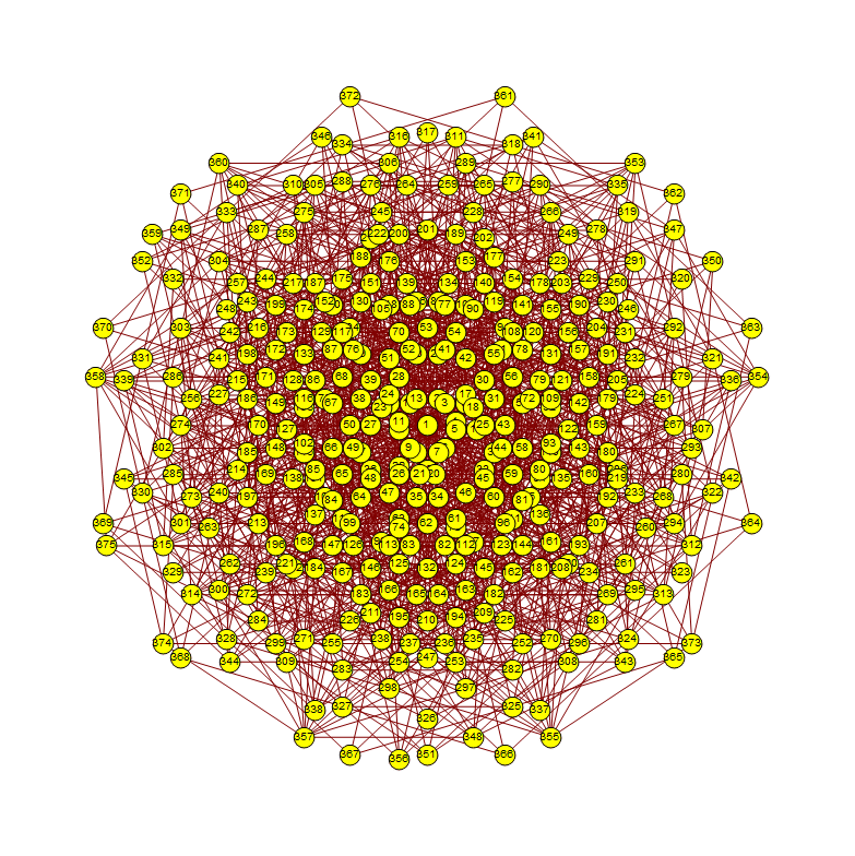
I was able to find some smaller unit-distance graphs with chromatic number 5. I started with my 529-vertex graph and reduced the large part and small part independently. For the large part I added all points in that are at unit distance with at least 6 points in the large part. Afterwards I applied the method as described in the article https://arxiv.org/abs/1907.00929 . The approach reduced the large part from 393 to 382 vertices. I found about a dozen different ones, but in most cases the graph is symmetric: it maps onto itself using a 120 degrees rotation. In earlier records, the large part was almost symmetric, but now it is fully symmetric. In a similar way I was able to reduce the small part from 137 vertices to 136 vertices. So the smallest graphs I have now have 517 vertices. The symmetric one has 2579 edges. A list of points and edges of this 517-vertex graph can be found in the repository at https://github.com/marijnheule/CNP-SAT .
That’s great! Congratulations!
Very cool Marijn! Yay for symmetry! Just for fun, try and find a totally symmetrical colouring?
Wait, I see a departure from symmetry. At the top, below the very top two vertices and just a scrap to the left of the y-axis, there are two yellow vertices very close together (in fact I think the right-hand one has x=0). 120o clockwise from there I duly see the same pair (they are red and green), but 120o anticlockwise I see only one: the one corresponding to the one with x=0 seems to be missing. What’s wrong?
Also there is an extra vertex near to where the missing one should be, in roughly the “5 o’clock” direction from there.
Correction – when I said “red and green” I meant “red and blue”
Another departure: at the bottom, there “should” be a vertex directly above the bottom red one, where the almost-vertical edge from the red one crosses an almost-horizontal edge. The vertices at the corresponding locations are both green.
It seems that only a large subgraph has 3-fold symmetry. The small subgraph is asymmetric. Maybe there is a symmetrical version?
I noticed another interesting thing: the 382-vertex graph (large part of 517er) is a subgraph of 2167er. That is, in fact, adding vertices is not required. Moreover, all the necessary orbits are already contained in the 529er and 525er.
I had earlier said that I wanted to make a video on my theorem on why coloring in 2 or more dimensions explicitly needs tiles. I missed the deadline back then and decided instead to polish up what I have a lot more, and I’m now finally done with that.
I’ve created a voiced and fully animated ~9 minutes video (using manim) where I’ve done my current best in getting my results across with as much visual intuition as possible.
I’m also going to use the same workflow I’ve established to make more videos on the other results in this thread. The next thing I’ll probably do is work on a video to give comprehensive visual understanding of the exclusion zone, effective exclusion zone, arc boundaries as well as the different tesselations we’ve explored. Aubrey and Jaan have contributed more than enough here for me to work with on that front for now.
If anyone thinks any specific concept in here could use some animated visualizations let me know.
Nice video. It would be interesting to see comments on it.
I tried again to understand the logic of your article. And although I still do not understand much, now I am at least able to formulate the question. I propose to limit to a flat case.
The exclusion zone is an zone in which one color is forbidden, namely, the color of the center of this zone. If the center is a point, then the forbidden zone is a circle. If the center is a continuous curve or region, then the exclusion zone has a nonzero area. It’s clear.
But I do not understand the concept of iterating of exclusion zones. It seems that here you substantially use the assumption that the entire exclusion zone or at least some of its continuous part must be colored by some single color, say red. This assumption is used in the next step of the iteration to generate a zone, which already has a nonzero area and cannot be colored red. Did I understand correctly?
Yes, but note that this assumption at first only works in very specific graphs, bipartite graphs. Because all vertices connected to a color 1 vertex can and have to be colored 2, and vice versa. That’s why a chromatic coloring of the integers requires all odd numbers to share a color, and all even numbers to share the other color.
In any bipartite graph, assigning a color to just one vertex explicitly locks down the coloring of the entire graph. They are rigid, just as complete graphs are.
2 n-balls at unit distance are such a bipartite graph. Placing any point of color in any of the 2 n-balls determines the full coloring of both. Iterating through the exclusion zones shows that. A point of color 1 in the first n-ball means the second n-ball has some connected vertices that can’t have color 1, and so have to have color 2, and then vice versa.
n-balls in such a way behave equivalently to single vertices. If you add a third n-ball connected to the former two then again the only way to get a chromatic 3-coloring is by giving each n-ball one exclusive color. From this a direct equivalence between n-ball graphs and finite graphs can be made.
The proof by contradiction here is, if we could chromatically color the plane, or higher dimensions, without using tiles, that is any continuous color, then we could do the same for n-ball subgraphs, which means 2+ colors for all n-balls. With n-balls being equivalent to vertices this would mean we could color the finite equivalents with 2+ colors per vertex, and finally, a bipartite graph too. Clearly however, if we have one vertex with colors 1 and 2, and it’s connected to another one, this other vertex can inevitably only have color 3. And 4. We’re using twice as many colors as we actually have to.
I previously thought there’s an argument for non-tile based coloring requiring infinite colors, but I’ve disproven this notion myself since. What’s explained above and in the video however shows that any non-tile based coloring will necessarily require more colors than a chromatic tile-based covering, meaning chromatic non-tile based colorings are just as much impossible as a chromatic 4-coloring of a bipartite graph is.
I suppose I could also make a second part to this video, where I dive into this with further explanations. It’s… not easy to judge which parts might cause hangups for others as I’ve worked on this for so long now. It’s no doubt similar to how many of the other concepts like computing fractional plane coloring here are deeply understood and now trivial to many of you, yet I have merely a cursory understanding of such.
What is n-ball?
Put simply a ball is the volume bounded by a sphere. A 1-ball is a line segment, a 2-ball a disk (such as the example in the video) and so on.
Is it assumed that the entire n-ball is necessarily colored in one single color?
If so, where does this assumption come from? Is it postulated or proved?
The hunt is in full swing. My shot: 510 vertices, 2508 edges.
https://www.dropbox.com/s/v5lbv5adropt2l0/v510e2508.vtx?dl=0
Large part of it, :
:
It is proven (as far as I’m concerned) for under specific circumstances. These circumstances being 2 such n-balls with the same radius at unit distance, such as in the video, where they are bipartite, containing no odd cycle.
The iteration shows this, as any single point of color determines the full coloring of both n-balls.
From there an equivalence between finite and n-ball graphs can be made.
Maybe. But this equivalence will only work as long as the balls are far enough apart. As soon as the distance between the boundaries of some two balls becomes less than their diameter, the equivalence will be violated.
Because in this case we will be able to place between two close balls a third one, which will be colored in at least two colors (as first two balls).
Jaan – he is specifying that the centres of the balls are exactly 1 apart.
Yes, but it doesn’t matter. Once many balls appear, one of them can fit just between the other two.
Jaan is correct, the radius will be heavily restricted in denser graphs. In the case of just n-balls the possible radius is 0.5. In the case of very dense graphs the possible radius can become arbitrarily close as vertices become arbitrarily close to having unit distance. The distance closest to unit distance is the limiting factor here.
However this also means that there’s always some radius possible, even if very small, under which the equivalence holds.
There is no such radius, since for any radius it is possible to construct a graph that is not equivalent to its counterpart from balls.
That’s correct, but there is also no need for one single radius to hold in all possible graphs. It’s entirely sufficient for any radius, even if extremely small, to work out in a specific given chromatic graph.
Taking for instance the Heule graphs this would proof that there is no 5-coloring of the plane without solid color. Using the De Bruijn–Erdős theorem we can tell that there is some finite graph in the plane with the same chromatic number. That graph will still allow some radius, proving up to that point, and thus for chromatic colors in general the need for some single colored volume. So there doesn’t need to be such a general radius.
On the contrary, there is such a need, at least it is essential for your proof. After all, in the end, you want to color the entire plane, and not a set of balls with gaps between them.
There needs to be only one working radius for one chromatic coloring.
As soon as there’s even one finite chromatic graph in the format such as the Heule graphs, that’d be all that’s needed for the theorem.
That’s because such a n-ball graph is a subgraph of the n-space. If the subgraph can’t be colored without some solid n-volume, then the main graph can’t be either.
If the main graph could be entirely colored without solid n-volume the same would have to be true of all subgraphs. All subgraphs including this one single case and radius for which it isn’t, thus no coloring without solid colors. Regardless of other subgraphs that would force a smaller radius.
There is another way of putting it too.
This would be a problem if and only if a finite chromatic coloring in euclidean spaces could only be made with 2 vertices having a distance arbitrarily close to 1, but not actually 1, so that they are not connected, and these two vertices would further explicitly need to have different colors.
This would also have to imply that chromatic colorings require vertex positions that can’t be expressed as any number, which I’m fairly certain is not the case.
Again I don’t understand anything. What is chromatic coloring? What is a graph format? Where exactly is the magical argument that shows the impossibility of coloring the plane without tiles?
So far I see the following chain of reasoning (correct me if necessary): 1. We take some specific finite graph. 2. We replace each of its vertices with a single-color ball of some small diameter. We call this construction a ball-graph (of a concrete initial graph). 3. We consider a generalization to the class of all ball-graphs. We implicitly make a statement that there exists a ball-graph covering the entire plane without gaps. 4. We apply the concept of exclusion zones to a generalized ball-graph. We conclude that tiles are necessary.
I see no reason for 3.
I see no reason for 3 either, that does sound rather impossible.
(Note I have answered what I mean with a chromatic coloring below in more detail.)
Here’s the actual chain of reasoning, I tried to really go into the details:
1. We take some specific finite graph, K2 to be exact, at unit distance, and turn the vertices into n-balls. We are looking only for chromatic colorings (as few colors as possible) which are 2 for K2, and we find this expanded K2 can only have single-colored balls. The behavior of this n-ball K2 to one another, for chromatic colorings and also in general, is equivalent to the finite K2. The exclusion zone here both shows us that the balls need to be single colored, and being in the exclusion zone of one another is equivalent to the edge of a normal graph.
We use this knowledge as a building block for further ball graphs the same as we do with normal finite graphs.
2. We construct a Moser spindle ball graph. We note that the Moser spindle contains a K2 ball graph. If we could color all balls in the Moser spindle without solid color while maintaining chromaticity of the coloring (that is no more than 4 colors), then we could also color the K2 ball graph without solid color while maintaining chromaticity. We previously already found we can not, some balls need to have solid color. 4 of the 7 balls need solid color. We find this is also equivalent to the finite case where in a given chromatic coloring, 1 of 3 vertices could be double-colored.
3. We consider a generalization to the class of all ball-graphs. Single-colored balls are to ball graphs what normal vertices are to normal graphs. Multi-colored balls are to n-ball graphs what multi-colored vertices are to normal graphs, meaning they are at best tolerable, at worst detrimental to searching for a chromatic coloring. No complete graph can have any multi-colored balls/vertices while also having a chromatic coloring with as few colors as possible. No graph can be made exclusively from multi-colored balls/vertices while having a chromatic coloring.
4. There exists a finite subgraph of the plane with the same chromatic number as the plane (De Bruijn–Erdős theorem). This graph can be expanded to its ball graph equivalent. This ball graph is still a subgraph of the plane. This ball graph requires some solid color to be colored with CNP colors.
It follows that the plane itself needs some solid color to be colored with CNP colors.
Wait. You say “If we could color all balls in the Moser spindle without solid color while maintaining chromaticity of the coloring (that is no more than 4 colors), then we could also color the K2 ball graph without solid color while maintaining chromaticity.” Why? All you showed with K2 was that disks are equivalent to points if you are using only two colours. You have not shown that they are equivalent if one has four (or even three) colours available.
Ah, wait – you also say “We previously already found we can not, some balls need to have solid color. 4 of the 7 balls need solid color.” What exactly do you mean there? What you have shown (correctly) is that for a certain colouring of the Moser spindle there are three “bichromatic vertices” as we have been calling them, i.e. vertices that can take either of two colours (so in your disk graphs, disks that can be speckled) if all six other vertices are monochromatic, but there are four that cannot because they have neighbours of all three other colours. But that doesn’t tell us what you want it to tell us, because you chose a particular colouring up front.
As far as only more colors are concerned we can show an arbitrary amount of colors to be directly impossible by considering complete graphs Kn with unit distances in (n-1)-space, including K3 in the plane. We know the subgraph K2 only works with 2 colors using solid regions. If we expand this to K3 this fact doesn’t change. Further if there are 3 colors within K2, then in the third ball of K3 there will be points excluded by all those 3 colors. Forcing the use of a 4th color, and thus us, again, to use more colors than the actual CN.
In regards to the equivalence, it is there and can be shown, it does however get some additional nuance. Multi-colored vertices are strictly speaking exactly equivalent to similarly truly multi-colored balls. Balls with speckling or local additional color aren’t quite the same, we see that as for the Moser spindle we can disperse the speckling.
This is also where measures come in again. Using measures makes the complete graphs up to arbitrary numbers and colors understandable, but it becomes complicated quickly beyond that. That’s an interesting direction, but not one needed for this proof I think.
Right. Monochromatic vertices are equivalent to monochromatic balls still. This follows from using balls and their shown traits as building blocks in the same way as finite vertices.
Bichromaticity is still equivalent, but with the additional nuance indicated in my previous post.
Go more slowly.
“As far as only more colors are concerned we can show an arbitrary amount of colors to be directly impossible by considering complete graphs Kn with unit distances in (n-1)-space, including K3 in the plane. We know the subgraph K2 only works with 2 colors using solid regions.”
Fine so far.
“If we expand this to K3 this fact doesn’t change.”
What fact doesn’t change? It’s true that we can’t colour the triangle of disks with two colours (at all, let alone with each disk monochromatic). But how do you do it with three colours? You can’t do your back-and-forth painting thing from the video, because the first curve (at 1 from the centre of a disk) need not be monochromatic.
“Further if there are 3 colors within K2, then in the third ball of K3 there will be points excluded by all those 3 colors.”
Again, please go more slowly. I agree that there must be three colours in any K2 of a triangle. But why must there be points in the third disk that are unit distance from all three colours?
“What fact doesn’t change?”
That we’ll use more colors than necessary.
“But why must there be points in the third disk that are unit distance from all three colours?”
Just for this instance let’s view this from the perspective of measures.
Each ball has a volume of v. In K2 we have 2 n-balls of some total volume 2v. Each ball in K2 excludes a minimum of volume v from having the same color.
Now, assume both balls are colored continuous, then the total color exclusion is 2v. Each v representing a color we get 2 colors.
If we add just a single point of a third color in one of these balls the total color exclusion will still be 2v + some additional exclusion from this additional point.
(This comes from the fact only boundaries count in regards to computing exclusion zones, not their insides. A differently colored point without the boundaries of a continuous other color is additional weight and nothing more.)
From the point of measures here we can see that we’re making a tradeoff without gain and we use more colors than necessary. The more we speckle, the more drastic this pointless tradeoff becomes.
(It also becomes computationally rather insane. Which is why I haven’t been able to formalize any of this beyond complete graphs)
In K3, we have 3 n-balls of some total volume 3v. Each ball in K3 excludes a minimum of volume 2v from having the same color. The total color exclusion is 6v. One full v per ball can overlap with another full v for 3v stacked exclusions. 6v-3v leaves 3v of necessary exclusion left to distribute among the volume 3v. 3 colors. Adding additional points here still gives us 3v + overhead, also forcing us into more colors.
That shows from a measure perspective that complete ball graphs have no flexibility for non-solid colored regions. I hope that’s understandable, but there’s more approaches to this too.
You keep introducing more and more machinery. That’s not good. I don’t think your new argument works (not easily, anyway): just looking at K2, yes if you flip just one point things get worse, but eventually you may get to the point where some points in the other disk become freer because you used the third colour for all the points that used to constrain them.
Assume we try to free up points.
In all Kn graphs like this there is an equivalently placed point in all balls. Let’s name the disks d1, d2 and d3. Assume an initial point of color 1, such as the center, in d1. Now there are some points in d2 that can’t have color 1. Pick on of those points, like the center again with color 2. Using equivalent center points those exclusion zones overlap in the center of d3 excluding colors 1 and 2 there. If we want a chromatic coloring this leaves us with only 3.
Now, if we tried to free up flexibility for a given point say the center of d1 with color1, this would mean having it excluded by less than 2 colors.
So only one color, either 2 or 3 among the 1-dimensional exclusion in both other balls. These excluded points have at the bare minimum one intersection among them, in this case the other center balls. This in turn forces the use of 2 colors in that 1-dimensional exclusion zone, and forcing us away from freeing anything up in this manner. This holds for all points in all balls. Thus we can’t free up a single point in this manner.
You can build an even more specific ball-graph containing only three balls. Let the coordinates of the centers of the balls be , where
  . We also fix the radius of these balls. We select 6 more points inside these balls, namely three points with coordinates
  and three points with coordinates
  . We choose
  and
and  so that the points are connected in the following order by unit distances: g_{0}-b_{1}-g_{2}-b_{0}-g_{1}-b_{2}-g_{0}. Color the points
  in green, the points
  in blue. How now to come to a contradiction, that is, to show that such a coloring is impossible?
Right. I too have been working in the context of the hypothesis that CNP=3 and trying to come up with a contradiction that only involves points within the three disks (as opposed to the cheat using a diamond), and I have not found one. Clearly in your (Jaan) construction it is possible to identify other points within the disks whose colour is forced, and I am reasonably sure that if any of the three disks is not monochromatic then they all need to feature all three colours, but that’s as far as I can get.
[You can build an even more specific ball-graph containing only three balls…]
I’ve upgraded my Python workspace to use your complex functions, since admittedly previously I simply used copypaste coordinates, to make sure I interpreted those functions correctly.
[I am reasonably sure that if any of the three disks is not monochromatic then they all need to feature all three colors, but that’s as far as I can get.]
I’m in turn reasonably sure that going down that route will lead to an infinite iteration that will never approach a full coloring without contradictions.
I mean, I assume there is a way to proof it thoroughly like that, making some math about calculating the limits of this type of iteration. Neither have I taken that route, nor would I want to introduce yet more machinery like that, nor do I frankly even have a rough guess of how to do it.
This thing has been a source of brain frying for me for a substantial amount of time as “probably infinite iteration that never approaches a proper coloring” is understandably highly unsatisfying and of not much worth in regards to a proof, and it’s also where I got stuck for months.
This is the direction I’m going instead. there is at least one explicitly not color flexible triplet of points
  .
.
For any complete unit distance n-ball graph the only condition under which speckling could maintain chromaticity is if more flexibility could be freed up with colors than is lost, as indicated by Aubrey here:
[…but eventually you may get to the point where some points in the other disk become freer because you used the third colour for all the points that used to constrain them.]
We will never get to this point however, as all points in all balls for any ball Kn in n-space are simultaneously part of at least one finite Kn, and no finite Kn coloring ever allows any color flexibility while maintaining chromaticity, this can be called categorically impossible.
For instance in K3 with a given offset o for every point
Not just do we not get enough flexibility to make up for the overexclusion caused by speckling, we can’t even get the tiniest bit for any point, no matter how far we iterate, as all it takes is one single triplet as above to show that we won’t free up anything in this direction.
If we could free up anything then this would imply that we can color K3, or for example the subgraph c_0, c_1, c_2 as defined in Jaan’s function with 2 colors, which is clearly not the case.
We know the proven fact K2 has 1 and only 1 chromatic coloring, which is a solid coloring, this K2 can be used as a building block for other ball graphs, including Kn. We can achieve chromatic colorings for any Kn in a similar fashion to K2, with solid regions.
We also know one coloring resulting in a chromatic coloring, and in regards to exclusion measure it fits with nothing to spare, and on the other hand we know speckling causes overexclusion with demonstrably no return in flexibility whatsoever, regardless of how far we iterate.
Rephrasing, if there was a way around it, we could color any Kn with colors appearing more than once per vertex. We can’t. That’s also a contradiction and what I would consider a proof.
A proof for complete ball graphs anyway. This holds for monochromaticity in general. With multichromaticity things get a bit of additional nuance as I implied earlier.
No. Think about it probabilistically. Every red point in disk A defines a curve of points in disks B and C that must be blue or green. But even if (wlog) at least 1/3 of the points in disk A are red, that still doesn’t tell us that every point in disks B and C is blue or green, because multiple red points in disk A can hit multiple points in disks B and C. Even if we say that at least 1/3 in disk A are red and at least 1/3 in disk B are blue, still we can only be sure of fixing 1/9 of the points in disk C to be green.
I have a strong sense that the people here who actually understand measurability and who have properly absorbed the Falconer paper could help us poor amateurs out here… anyone?
[…who have properly absorbed the Falconer paper…]
Yeah that’s admittedly not me.
[Even if we say that at least 1/3 in disk A are red and at least 1/3 in disk B are blue, still we can only be sure of fixing 1/9 of the points in disk C to be green.]
I don’t think that works, but I’ll take a step back now and instead ask something myself. If we’re going probabilistic I might be out of my water so I’m not near as certain about this.
First, think back to K2. As I’ve shown placing a single point in either ball locks the entire coloring, in this special case however it does never actually reach a last step, as we only get arbitrarily close to the boundaries of the balls along their shared axis.
There are however at least 2 configurations of merely 1-dimensional sets of points that will instantly snap the entire coloring into place with just 2 iterations.
One of them is the boundary of a ball. The boundary itself has the same exclusion zone as the entire ball itself. So if the boundary of one ball was solid red, this in and of itself would prevent any and all red from appearing in all other balls. The inside of the ball doesn’t even matter anymore. 100% 1-Dimensional boundary coloring gives us 100% n-Dimensional ball exclusion.
Similarly a line crossing through the center of one ball, pointing to another ball also excludes the entirety of that ball. And a fair bit extra in other balls too.
Now if the colors are finely dispersed that means the boundaries of 2 disks, say A and B both contain 1/3 red, as well as the lines within disk A and B pointing at disk C also contain 1/3 red. Any such solid boundary or line by itself would produce 100% exclusion. I guess we would then assume 1/3 of that produces 1/3 exclusion, right?
How are 4 patterns with (at least) 1/3 exclusion going to add up to no more than 1/3 exclusion still?
And that putting aside the fact that with just the outer boundary and a single line in 2 balls we are considering an infinitely small part of the actually red colored points? Is there any way this can work probabilistic?
Sorry, I have to correct myself on that last part.
How are 4 patterns with (at least) 1/3 exclusion going to add up to no more than 2/3 (instead of 1/3) exclusion still?
The spare points after this are of course still a thing.
I’m not even sure how you got the 1/9, I don’t see why these things should multiply. Probably knowing what disks A, B and C are would help.
Anyhow, I think that this debate about Bernhard idea is getting too long. The original idea and video seem to lack the rigorousness required from a mathematical proof, and since no one seems to understand it, I think we should wait until Bernhard can post a version that is more mathematically founded, and then we can return to it.
Hi Domotor,
That wasn’t my request. I am very sure, and so is Jaan, that Bernhard does not have a solid proof that MCNP = CNP, in my case mainly because if there were so simple a proof then I’m sure it would have been found long ago. However, we are unable to formulate a clear description of why it is actually really hard to prove that MCNP=CNP. Bernhard’s attempt is not really relevant here. Even sticking to chromatic number 3, neither Jaan nor I can construct an explicit 3-colouring of disks of small radius and centres (0,0), (1,0) and (1/2,Sqrt[3]/2) that avoids unit distance; but neither can we construct a proof (a rigorous proof, unlike Bernhard’s) that no such colouring exists. Hence, we are at the mercy of this thing called Lebesgue measure that is used so freely in Falconer and elsewhere. Extensive rumination on the definition of it at Wikipedia has not helped me to gain a precise understanding of what it really is, nor even an understanding of how “having measure greater than 0” differs, in relevant ways, from “being bounded by a Jordan curve”. For example, it is clear to me that we can say a lot more about colourings of R^2 that have even one continuous monochromatic curve in them than about colourings that do not, even though as far as I can tell such curves have zero measure in R^2.
Therefore, my humble request is to explain the logic of Falconer in terms that do not assume an understanding of measure.
That leaves the question what kind of proof is desired here. I’ve stuck with using generally proven traits of graphs and their subgraphs and making equivalence relations from those on n-ball graphs, as that’s also where this pretty much has to end up to be actually useful.
I have studied into Lebesgue measures as well, although not very deep. I got sidetracked just about long enough to make an equivalent experiment in non-unit distance 1-Dimensional graphs, which has worked out using ordinal arithmetic. Thus I stuck with the measures just about long enough for the K2 case. Not beyond that.
That’s why I brought up that the boundary itself as well as pointing lines exclude all points in other balls by themselves. If you think a probabilistic proof of that is going to help my case, then I suppose that’s where I’ll go.
I’m joining to Aubrey’s request. And it’s probably better to start a new chain for this.
I would be curious about that too but I have my reservations about whether such can be reasonably rephrased without an understanding of measures.
I do have another approach using directed lines and measures that reliably “chops off” 1/3 of the leftover coloring room in a different ball (so multiplicative 2/3), but I’ll just look it over some more times, post the full thing in some days or so if I don’t find anything wrong with it. I don’t see a reframing of this however that doesn’t use measures, except trying to put the whole thing into percentages.
In the meantime something wholly different:
[…nor even an understanding of how “having measure greater than 0” differs, in relevant ways, from “being bounded by a Jordan curve”.]
There are things with a measure greater than 0 that can’t be properly described by just a Jordan curve, or Jordan-Brouwer space separation in the more general case.
An example of this is the Smith–Volterra–Cantor set, a nowhere dense set with positive measure nonetheless. There’s also curves with positive measure themselves, such as the Osgood curve which can be a Jordan curve, as well as other space-filling curves (Peano, Hilbert, Lebesgue, Moore…), which have any desired positive measure but are often not Jordan curves at all (are self-intersecting).
I think it’s a good idea to start a new thread, but please one of you should define the question as a starter; constructing an explicit 3-colouring of disks of small radius and centres (0,0), (1,0) and (1/2,Sqrt[3]/2) that avoids unit distance seems trivial – just color each ball with a different color. Are you looking for a different coloring?
Also, another set of full measure that is not bounded by the Jordan curve is the set of irrational numbers. I think that we should be careful with non-measurable colorings; a nice example is given in Monsky’s theorem: https://en.wikipedia.org/wiki/Monsky%27s_theorem
[Are you looking for a different coloring?]
A non-tile based coloring. I’m arguing that such a coloring does not exist, and that only the solid coloring you mention works. That case is proven beyond doubt for disk K2. The question is up for disk K3 and other graphs, and a proof for that is the goal.
I see! Well, I think that this is probably open. I’ve asked a somewhat related question on Mathoverflow one year ago and I didn’t receive any answers: https://mathoverflow.net/questions/304966/can-a-big-set-always-look-small This older question I’ve linked to is even more related: https://mathoverflow.net/questions/108507/a-kakeya-like-problem-must-a-union-of-annuli-fill-the-plane
Yes, these look related and I should be able to work myself into them at least a bit the next days, might help me pinpoint things that I need to be aware of, figure out and clarify with the measure approach I intend to use. particularly the fat cantor thing in the second question sounds very relevant.
Say, when I’d ask you about the dimension and measure of a fat cantor set of perpendicular lines, could you confidently answer this? Say a fat cantor set of total measure 1 and dimension 1, made of perpendicular lines of measure 1 and dimension 1? I’d say that should still be measure 1 but dimension 2, is that right?
(Sorry of the terminology isn’t right, I hope the point comes across anyway.)
And does the Marstrand proof you mention in the second thread count for totally disconnected sets such as fat cantor too?
Yes, it would be measure 1 w/r/t the two-dimensional Lebesgue measure.
Thanks a lot for these pointers. Using this in combination with my previous iterative work I see a way to make a purely measure and percentage based iterative function that’ll show that the act of attempting to fully speckle any ball in a ball graph will exclude that color necessarily from any connected balls. Unlike the bipartite example which only works explicitly in K2 this seems to work for any arbitrary ball in any ball graph with any number of colors. Not just that… it actually explains much better than anything I had before how multichromaticity works in ball graphs, it seems to establish the missing equivalence.
I’ll get on it and post it in the 14th thread in a few days, and with that I’ll sign off permanently from this too-long-subthread. Unless one of the others has a new thread starter this can be it once I’m done.
Also so this doesn’t get buried, what Aubrey requested earlier:
[Therefore, my humble request is to explain the logic of Falconer in terms that do not assume an understanding of measure.]
Hi Bernhard,
I’ve just had a look at your video. It is a very nice presentation!
I think I see a gap in your proof, though. Around 6:10, when you draw the curve inside one disk that is 1 away from the centre of the other disk, you set up a nice argument for why the two disks must each be just one colour in a 2-colouring. But if you were allowing three colours, the curve need not be one colour, nor even a sequence of measurable segments of one colour: for example if the centre of the left circle were red, the curve in the right circle could be blue for rational values of the y-coordinate and green for irrational values. I think that ends up allowing both disks to be speckled, and I don’t see a way to tweak your construction to avoid this.
Exactly this type of speckled coloring is what I realized myself a few weeks ago which thoroughly disproved my topological attempt at proving the necessity of tiles and infinite colors without tiles. A finite coloring with such speckling is certainly possible.
However chromaticity is the key here to the proof. It is not possible to speckle the n-balls while still having a chromatic coloring and the proof is only concerned with chromatic colorings, thus the third color is ruled out. That’s what makes 2 such n-balls at a certain radius (even when very small) equivalent to 2 finite vertices.
It is also explicitly possible to have some volume speckled like this in some chromatic colorings for non-complete graphs, and most likely a whole plane coloring. You can see when and how this speckling becomes possible (although useless) in the video at 2:42 and 6:56.
At 6:56 thus you can speckle one of the 3 marked n-balls without losing chromaticity, and depending on how you do it you can also disperse the speckling (or a different solid color, or a double color) throughout the 3 n-balls. However I’m fairly certain you’ll find it as impossible to speckle all n-balls in an n-ball Moser spindle as you will in the 2 n-ball case.
That’s also all the theorem is supposed to proof. That some area can not be speckled, and that speckling is generally not of any use for a chromatic coloring.
What do you mean by “chromaticity” and “a crhomatic colouring”?
As in using the chromatic number of colors to color something, not more colors. We could for example color the Moser spindle with 7 colors if we gave each vertex its own color, but that number and coloring isn’t what we’re looking for here. We’re looking for a coloring with the fewest colors possible, which for the Moser spindle is 4 not 7. We could even put in an arbitrary amount of colors by using multiple colors per vertex, but that’s also not what we’re looking for.
Such a 4 coloring I would call a chromatic coloring. A coloring using more colors than needed I’d call a non-chromatic coloring. If there’s some better terminology I’m missing let me know.
OK, thanks. So let me be clear: are you claiming to have proved that there is a tiling of the plane with N colours where N is the CNP? Equivalently, that if there is no 6-tiling of the plane then CNP=7 ?
I’m trying to extend your logic more explicitly to more than two colours. I can do it for three colours (using three disks in a triangle), but only by using a fourth set of points: specifically, since if we use only three colours we know that a diamond has its opposite corners the same colour, we can say that any curve at constant distance Sqrt[3] from the centre of a disk is all the same colour as that disk, and that lets us do an iterative painting argument analogous to what you give for two disks. And that doesn’t extend to four colours unless we cheat, by making use of our knowledge that 4-chromatic graphs exist in which two specific vertices (at distance 8/3) are always the same colour. I don’t see any other way to do your painting thing with more than two colours. Please spell it out. All you have said so far is that in your chosen colouring of the Moser spindle there are some vertices (hence disks) that can be speckled if all the others are monochromatic, but you have not addressed the possibility of all seven of them being speckled.
As I’ve replied above now I’ll just address the 6-tiling case. It’s correct that, if my theorem holds, that the absence of a 6-tiling would imply CNP=7.
Not that Coulsons “On the chromatic number of plane tilings” does not mesh with ball graphs to prove that the CNP is 6 or 7, as Coulsons approach assumes convex tiles, which the ball graphs to not imply at all.
My message was lost or the moderator delayed it for more than a day. I repeat it without pictures.
There are 5-chromatic graphs with 510 vertices. All files are in the polymath project dropbox.
Yay! I was wondering, because the graph appeared in my dropbox but there was no post.
It is becoming more and more important that you write up a detailed description of your method. Are you working on that?
I did not forget about the promise to describe my method of graph reduction. It is actually based on brute force. But there are many ways to speed up it.
The method is still under development. There is a possibility that it will not be finalized until the end. Competition is more exciting than tedious work. And now I’m tired of the competition. Now I use short routines in Mathematica, many operations are performed manually. The program can be accelerated at least 100 times, but so far this does not make much sense. I spent less than two days to find the extra 7 vertices.
And it’s not yet clear to me whether it is worth wasting time on a detailed description. I would first wait for the return shot from Marijn.
Ha! Well, I do agree that the competition is fun (also for the spectators!), but on the other hand, since you and Marijn are using each other’s advances as steps to your own, it seems very likely that there could be more progress by combining the methods than by bouncing graphs back and forth. In particular, it would be great if you could have access to Marijn’s code so that you could apply his methods “on demand” to your graphs. I understand that it may not be possible to do the reciprocal, if a lot of your method is manual. Do you already have his code, or some of it?
Our approaches differ significantly. I feel that Marijn’s approach is more stochastic, my more deterministic. Marijn uses a special tool, DRAT-trim, I don’t use. I also tried it, but did not get any impressive results. Most likely, because I do not have large computing power.
An interesting question, could I get at least the same 510-vertex graph without having Marijn’s graphs as a starting point? (Note that Marijn most likely did not use my results.) I am not ready to answer it, for this I have to go all the way again, for example starting from my 451-vertex graph. Theoretically, my method allows to do this. Because it is gradually becoming smarter.
I have no convenient code. There is not even a clear understanding of a successful search strategy. There is only a set of procedures, a bunch of scribbled paper, some experience and many ideas. In general, the method is still crude.
Fair enough. That makes your achievmeents all the more impressive!
That’s a whole 43 vertices down from the sample I used in my video, nothing to scoff at. And it’s not just interesting to watch, smaller graphs are also so much nicer for visualization and animation without having… 2000+ vertices or something.
Though I guess with 6 colors that’s how it will ultimately look anyway.