Compressed Sensing and its Applications 2015

Last week, I attended this conference in Berlin, and much like the last CSA conference, it was very nice. This year, most of the talks followed one of three themes:

Application-driven compressed sensing
Quadratic or bilinear problems
Clustering in graphs or Euclidean space

Examples of application-driven CS include theoretical results for radar-inspired sensing matrices and model-based CS for quantitative MRI. Readers of this blog are probably familiar with the prototypical quadratic problem (phase retrieval), and bilinear problems include blind deconvolution and self-calibration. Recently, I have blogged quite a bit about clustering in Euclidean space (specifically, k-means clustering), but I haven’t written much about clustering in graphs (other than its application to phase retrieval). For the remainder of this entry, I will discuss two of the talks from CSA2015 that covered different aspects of graph clustering.

— Background —

Consider a random graph following the inhomogeneous Erdos–Renyi model $G(n,(p_{ij}))$ . Here, vertices $i$ and $j$ share an edge with probability $p_{ij}$ , independently of the other edges. For example, in the stochastic block model, the vertices are partitioned into $k$ communities, and then $p_{ij}$ equals either $p$ or $q$ according to whether $i$ and $j$ are members of the same community:

sbm1

(Figures courtesy of Afonso Bandeira.) Now suppose you receive an instance of this random model, but you are not given the partition into communities (or $p$ or $q$ ):

sbm2

The goal of community detection is to estimate the communities from this data. Consider the special case where there are $k=2$ communities, each of size exactly $n/2$ . It turns out that if $p$ and $q$ scale like $(\log n)/n$ , then exact community recovery is possible, and the phase transition is well understood. (Intuitively, this makes sense since the signal is given in the form of connectivity, and $(\log n)/n$ is the ER threshold for connectivity.) If $p$ and $q$ scale like $1/n$ , then exact recovery is impossible, but there’s also a well-understood phase transition for when you can estimate better than random guessing. (Here, $1/n$ matches the ER threshold for a giant component.)

Given a graph with adjacency matrix $A$ , consider the normalized graph Laplacian:

$\mathcal{L}(A)=I-D^{-1/2}AD^{-1/2},$

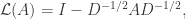
where $D$ denotes the diagonal matrix whose $(i,i)$ th entry is the degree of the $i$ th vertex. The eigenvalues of $\mathcal{L}(A)$ lie between 0 and 2, and it’s easy to verify that $D^{1/2}1$ is an eigenvector with eigenvalue $0$ . The dimension of the null space equals the number of connected components in the graph, and in fact, the null space is spanned by vectors which are supported on each of the components. Intuitively, the graph is well connected if the second-smallest eigenvalue is large (as exemplified by Ramanujan graphs), and if this eigenvalue is small but the third-smallest is large, then your graph is essentially two well-connected components with a few edges added to connect the two (much like the stochastic ball model with $p$ large and $q$ small). In this case, the second eigenvector is “close” to being in the null space, and so the two well-connected components can be determined by finding a couple of localized vectors that span the span of the first two eigenvectors (in practice, it suffices to take the sign pattern of the second eigenvector). This is called spectral clustering.

— Recovering hidden structures in sparse networks —

Roman Vershynin gave a talk based on two papers (one and two). Here, we will discuss the first paper. Suppose you want to perform spectral clustering to solve community detection under the stochastic block model. In order for this to work, you might expect it to necessarily work for the “expected graph,” whose normalized Laplacian is easily computed as

$\displaystyle{\mathcal{L}(\mathbb{E}A)=I-\frac{1}{n}11^\top-\frac{p-q}{p+q}\frac{1}{n}vv^\top,}$

where $v$ denotes the vector which is +1 for vertices in the first community and -1 in the second. Indeed, the second eigenvector of this expected Laplacian is $v$ , as desired. In order for this behavior to be inherited by the random graph, we would like its eigenstructure to be close to its expectation. By the Davis–Kahn theorem, it suffices for $\mathcal{L}(A)$ to be close to $\mathcal{L}(\mathbb{E}A)$ in the spectral norm. As such, we seek some sort of concentration phenomenon.

It is known that the Laplacian exhibits such concentration in the “dense” regime where the $p_{ij}$ ‘s scale like $(\log n)/n$ . On the other hand, the “sparse” regime (where the scaling is $1/n$ ) is flooded with isolated vertices, and so all of these components thwart the success of spectral clustering (let alone Laplacian concentration, which would imply success). A similar problem was encountered in the development of PageRank: Since the internet has many isolated pages, a random surfer would fail to reach these pages, and so the surfer model is modified to allow for a small probability of “getting bored” (in which case the surfer visits a webpage drawn uniformly at random). This modification to the surfer model can be interpreted as a modification to the graph, where every pair of vertices receives an additional edge with appropriately small weight. If the added weights are selected appropriately, it turns out that this regularization allows for concentration in the Laplacian:

Theorem (Theorem 1.2 in Le–Vershynin). Pick $\tau\sim d:=\max_{ij}np_{ij}$ and define the “regularization” $A':=A+(\tau/n)11^\top$ . Then

$\|\mathcal{L}(A')-\mathcal{L}(\mathbb{E}A')\|_{2\rightarrow2}=O(1/\sqrt{d})$

with high probability.

The proof of this result amounts to iteratively finding a decomposition of the adjacency matrix using a neat Grothendieck-type inequality:

Theorem (Grothendieck–Pietsch factorization). Let $B$ be a $k\times m$ real matrix and $\delta>0$ . Then there exists a $k\times l$ submatrix $B'$ of $B$ with $l\geq(1-\delta)m$ such that

$\displaystyle{\|B'\|_{2\rightarrow 2}\leq\frac{2\|B\|_{\infty\rightarrow2}}{\sqrt{\delta m}}.}$

By iteratively applying this inequality, one may isolate portions of the matrix which are sufficiently dense (from a spectral perspective) to concentrate “for free,” and then the remaining sparse portions (which are more significantly impacted by regularization) may be estimated by Riesz–Thorin interpolation.

Some open problems along these lines:

Le–Vershynin regularize with $\tau\sim d$ , but what is the optimal parameter?
Can $\max_{ij}np_{ij}$ be replaced by $\max_i\sum_jp_{ij}$ ?
Does regularization find applications with more general random matrices?

(For the last problem, regularization does bear some resemblance to the truncated spectral initialization of the new Wirtinger Flow paper.)

— Phase transitions in semidefinite relaxations —

Andrea Montanari also gave a talk based on two papers (one and two), and we will discuss the first one. This talk investigated the advantages that SDP clustering has over spectral methods. Given a random graph of average degree $d$ , consider the following SDP:

$\mathrm{SDP}(A-(d/n)11^\top)~~:=~~\max ~~\langle A-(d/n)11^\top,X\rangle ~~\mathrm{s.t.} ~~\mathrm{diag}(X)=1, X\succeq0.$

Clearly, the value of this program is a function of $A$ . The main result of the first paper is that thresholding this value will typically distinguish stochastic block model graphs with edge probabilities $p=a/n$ and $q=b/n$ from ER graphs with constant probability $(a+b)/(2n)$ when

$(a-b)^2>(1+o_{a+b}(1))\cdot 2(a+b).$

For reference, it is known that there is not enough signal for any test to succeed when $(a-b)^2<2(a+b)$ . By comparison, performing spectral clustering to the regularized graph will work when $(a-b)^2>C(a+b)$ for some unreported constant $C>0$ (see equation (1.7) in Le–Vershyni).

To prove this result, one must find upper and lower bounds on $\mathrm{SDP}(A-(a+b)/(2n)11^\top)$ in the cases where $A$ comes from the stochastic block model and the ER model, respectively. To estimate this value, Montanari and Sen use a Lindeberg-type method to pass the random models to analogous Gaussian models, for which the desired tail bounds are more accessible.

I personally find the Lindeberg method to be quite interesting. The main idea is that, if $f\colon\mathbb{R}^n\rightarrow\mathbb{R}$ is smooth, $X$ is a random vector with iid entries of mean 0 and variance 1, and $Y$ is a random vector with iid Gaussian entries of mean 0 and variance 1, then $\mathbb{E}f(X)$ is close to $\mathbb{E}f(Y)$ . In fact, the entries of $X$ need not be independent, but rather exchangeable (see Theorem 1.2 in Chatterjee). This method was recently leveraged by Oymak and Tropp to study a particularly general class of random projections.

In order to leverage Lindeberg to convert to Gaussian, we need a smooth function, but considering how pointy the PSD cone is, it comes as no surprise that $M\mapsto\mathrm{SDP}(M)$ fails to be sufficiently smooth. To remedy this, Montanari and Sen first define

$\mathrm{OPT}_k(M)~~:=~~\max ~~\langle M,X\rangle ~~\mathrm{s.t.} ~~\mathrm{diag}(X)=1, X\succeq0,\mathrm{rank}(X)\leq k.$

Then each $X$ in the feasibility region can be expressed as a Gram matrix $\sigma^\top\sigma$ , where $\sigma\in\mathbb{R}^{k\times n}$ and each column has unit 2-norm. Of course, $\mathrm{OPT}_n(M)=\mathrm{SDP}(M)$ , and a symmetric version of Grothendieck’s inequality, gives that $\mathrm{OPT}_1(M)\geq(C/\mathrm{log}~n)\mathrm{SDP}(M)$ . Montanari and Sen generalize this inequality to show that $\mathrm{OPT}_k(M)\approx\mathrm{SDP}(M)$ for each $k$ .

However, $M\mapsto\mathrm{OPT}_k(M)$ is still not a smooth function, but it can be approximated by a smooth function by leveraging ideas from statistical mechanics. Indeed, consider the log-partition function

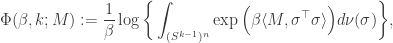
$\displaystyle{\Phi(\beta,k;M):=\frac{1}{\beta}\log\bigg\{\int_{(S^{k-1})^n}\exp\Big(\beta\langle M,\sigma^\top\sigma\rangle\Big)d\nu(\sigma)\bigg\},}$

where $d\nu(\cdot)$ denotes the uniform measure over the product of spheres $(S^{k-1})^n$ . As $\beta$ gets large, the integrand becomes increasingly peaky at the maximizer of $\mathrm{OPT}_k(M)$ , and so the log approaches $\beta\mathrm{OPT}_k(M)$ . As such, $\lim_{\beta\rightarrow\infty}\Phi(\beta,k;M)=\mathrm{OPT}_k(M)$ , suggesting that one may pick $\beta$ so as to juggle smoothness and approximation.

One thought on “Compressed Sensing and its Applications 2015”

rajeshd007 says:

January 19, 2016 at 5:34 am

An interesting post by me, related to compressed sensing : https://rajeshd007.wordpress.com/2016/01/19/a-concept-in-classical-fourier-analysis-and-its-similarity-to-compressed-sensing-using-minimum-total-variation/

	Jaan Parts on Polymath16, seventeenth thread…
	Jaan Parts on Polymath16, seventeenth thread…
	Jaan Parts on Polymath16, seventeenth thread…
	Jaan Parts on Polymath16, seventeenth thread…
	Jaan Parts on Polymath16, seventeenth thread…
	Jaan Parts on Polymath16, seventeenth thread…
	Jaan Parts on Polymath16, seventeenth thread…
	Tom Sirgedas on Polymath16, seventeenth thread…
	Jaan Parts on Polymath16, seventeenth thread…
	Tom Sirgedas on Polymath16, seventeenth thread…
	Tom Sirgedas on Polymath16, seventeenth thread…
	Jaan Parts on Polymath16, seventeenth thread…
	Tom Sirgedas on Polymath16, seventeenth thread…
	Tom Sirgedas on Polymath16, seventeenth thread…
	Tom Sirgedas on Polymath16, seventeenth thread…

Share this:

Like this:

Related

One thought on “Compressed Sensing and its Applications 2015”

Leave a Reply Cancel reply