
This is the sixteenth “research” thread of the Polymath16 project to make progress on the Hadwiger–Nelson problem, continuing this post. This project is a follow-up to Aubrey de Grey’s breakthrough result that the chromatic number of the plane is at least 5. Discussion of the project of a non-research nature should continue in the Polymath proposal page. We will summarize progress on the Polymath wiki page.
The paper writing has found a second wind between Philip Gibbs, Aubrey de Grey, Jaan Parts and Tom Sirgedas. For reference, I wanted to compile a list of related publications that have emerged since starting our project. (Feel free to any references I missed in the comments.) There has certainly been a bit of activity since Aubrey’s paper first hit the arXiv two years ago!
P. Ágoston, Probabilistic formulation of the Hadwiger–Nelson problem.
F. Bock, Epsilon-colorings of strips, Acta Math. Univ. Comenianae (2019) 88: 469-473.
J. Parts. A small 6-chromatic two-distance graph in the plane, Geombinatorics, vol. 29, No. 3 (2020), pp.111-115.
J. Parts. Graph minimization, focusing on the example of 5-chromatic unit-distance graphs in the plane, Geombinatorics, vol. 29, No. 4 (2020), pp.137-166.

Repost of my latest offering regarding Jaan’s 6-tiling:
Thanks Jaan! But I’m still not reproducing this.
I agree with you about Mathematica – I too am using FindMaximum and being careful about ranges.
If we orient things following Pritikin and place the centre of a diamond at the origin, then here is my notation:
– the sharp corners of that diamond are at (0,+/-d)
– the blunt corners of that diamond are at (+/-e,0)
– the tip of the arrowhead at y=0 is at (c,0)
– the back of that arrowhead is at (b,0)
– the “trailing tip” of that arrowhead is at (r,s)
– the back of the arrowhead at y=1/4 is at (g,1/4)
Then we have four distinct diameters of large tiles, which give the constraints:
(c-e)^2 + (1/2)^2 is at most 1
g^2 + (1/4 – d)^2 is at most 1
(r-e)^2 + (1/2 – s)^2 is at most 1
(b+g-r)^2 + (1/4 + s – d)^2 is at most 1
with all seven values positive, and with c,b,r,g in increasing order and less than 1. In practice d,e,s are less than 0.1 and g,r,b,c are more than 0.8.
Also we have a “Bock-esque” situation in the neighbourhood of ((b+g)/2,3/8), where two large tiles meet that need to be 1 away from tiles on the far side of relevant diamonds, giving:
(b+g)^2 + (3/4 + 2*d)^2 is at least 4
(b+g+e)^2 + (3/4 + d)^2 is at least 4
(b+g+2e)^2 + (3/4)^2 is at least 4
This is all without curving any edges of diamonds or arrowheads, but you said that that makes only a small difference (6899 to 6906). Undulation of the inter-arrowhead edges is needed (at least if any of the things that are >=4 are exactly 4), but does not introduce any additional constraints.
So, I’ve hunted around the search space and the best I have is this:
{6690.97, {d -> 0.0124893, r -> 0.873218, b -> 0.872363,
c -> 0.871225, g -> 0.971385, e -> 0.00519998, s -> 0.00346665}}
But I think I must be missing your sweet spot, because with this setup we have
(b+g+e)^2 + (3/4 + d)^2 = 4
which means that the edges of the diamonds must curve OUTWARDS, as I said in my earlier post, which means they will not be 12-gons as you say.
Why don’t you want to try 12-vertex diamonds? For example, we add a pair of vertices (i, f) and (j, h). In this case, the set of constraints will change, and instead of (0, d) and (e, 0) in >=4-constraints there will be new vertices.
My reasoning is that the only situation in which the addition of a vertex will help is when the line (or arc) that it would bisect is not already constrained, i.e. in which some part of it it could be curved (or its radius of curvature changed) in either direction without creating a unit-distance pair of points. In the best construction I’ve found, the edge of a diamonds is an arc of radius 2 that is exactly 1 from an arc of radius 1 that forms part of an inter-arrowhead boundary between two large tiles. Thus, it can only be made more curved, not straighter.
Not sure I understand your reasoning. I can answer so. First of all, you cared about pulling distant tiles to a distance of 2. This is correct. But there is another task: to make the tiles more convex. This can give an increase in the fraction of the colored plane. And this is achieved using 12-vertex diamonds. How about such a reasoning?
The problem is that in this case the curvature makes the DIAMONDS more convex, i.e. it makes the diamonds bigger and DECREASES the fraction of the plane that is covered by the big tiles. The only way that this could be advantgeous is if there is an accompanying reduction in the size of the arrowheads – but there isn’t, because their vertices (and edges) are constrained by the vertices of the diamond, i.e. by d and e in my notation.
In my case diamonds are non-convex.
OK. I’d better show my solution. Although it would be better to wait for the picture.
Consider a 15-gon whose vertices are numbered counterclockwise from 1, starting at your vertex (0, d). But I will use my notation. In fact, we need to consider the 19-gon, but for now we will not pay attention to the wavy inclined edges. Due to the symmetry of the 15-gon, it is enough to consider one “diagonal”, as in your case. We get the following restrictions: 16 distances between vertices 1…4 and 8…11 should be no more than 1 (you can remove some of these constraints, but we will be not greedy). The distance between the distant edges 2-3 (in contrast to yours 1-4 in my notation) should be at least 2, while these edges themselves must be parallel.
It remains to introduce some variables and express through them the coordinates of the vertices 1…4 and 8…11. I used the following notation:
{(0,a), (f,b), (f_2,b_2), (c,0), … , (h-l_2,w/2), (h-2d_2(h-g)/w,w/2+d_2), (g+2d(h-g)/w), (g-l,w), …}
Here g, h, w are macro parameters (describing the base 5-gon), the rest are small values (describing corrections). (I will replace these notations in the future, they just appeared historically.) Here is the solution vector:
{6985.43, {a->0.013326, c->0.005483, b->0.010031, f->0.000820, b_2->0.003322, f_2->0.003590, g->0.872081, h->0.972098, l->0.000572, d->0.003276, l_2->0.000509, d_2->0.003290, w->0.500000}}
Thanks. Couple of questions:
1) There is a y-coordinate missing in “(g+2d(h-g)/w)”. Should it be “w-d_2”?
2) “d” appears only in “(g+2d(h-g)/w)”. Should “h-2d_2(h-g)/w” actually be “h-2d(h-g)/w”?
I’m assuming yes to both.
OK, so the mapping from your variables to mine is as follows, where I have written your variables in capitals and mine in lower case:
A = d
C = e
H-L_2 = g
H-2D(H-G)/W = b+g-r
D_2 = s
G+2D(H-G)/W = r
G-L = c
So then, inserting your numbers I get:
d = 0.013326
e = 0.005483
s = 0.003290
c = 0.872081 – 0.000572 = 0.871509
g = 0.972098 – 0.000509 = 0.971589
r = 0.877412
b = H+G-g = 0.872590
But when I calculate the relevant distances, I get two diagonals that are more than 1:
(0,a) to (h-l_2,w/2) comes out as 1.00099
(c,0) to (g+2d(h-g)/w,w-d_2) comes out as 1.00698
I’m pretty sure this is not just a significant-digits issue.
I’m sorry: missed coordinate is (g+2*d(h-g)/w, w-d). Parameters d and d_2 are slightly different.
Now my check (where you get more than 1):
(0.972098-0.000509)^2+(.25-0.013326)^2 = 1
(0.872081+2*0.003276(0.972098-0.872081)/.5-0.005483)^2 + (.5-0.003276)^2 = 1
Thanks, but wait, in that case your arrowheads are not all the same – the one at w/2 is slightly taller than the one at w, since d_2 is slightly larger than d – which is not allowed.
First: I am assuming that the tile whose vertices you are enumerating has symmetry across y=w/2, so that the vertices you have not listed are (0,w-a), (c,w), (h-2d_2(h-g)/w,w/2-d_2), (g+2d(h-g)/w, d) and (g-l,0). Right?
Now, consider the big tile on the other side of the (h,w/2) – (g,w) line. What are the coordinates of its vertices? I can see only two possibilities, depending on what you do with l and l_2: either there are vertices at (g+l, w), (h+l_2, 3w/2) and (h+l_2, w/2) or else at (g+l_2, w), (h+l, 3w/2) and (h+l_2, w/2). In both cases, the other vertices are (h-2d_2(h-g)/w, w/2+d_2), (g+2d(h-g)/w, w-d), (g+2d(h-g)/w, w+d), (h-2d_2(h-g)/w, 3w/2-d_2), (h+g-c, 3w/2), (h+g, 3w/2-a), (h+g, w/2+a) and (h+g-c, w/2). And that’s a problem, because effectively d and d_2 have been swapped (whether or not l and l_2 have also been swapped), so you have some diagonals >1. In particular, (h+g-c, 3w/2) to (h-2d_2(h-g)/w, w/2+d_2) is 1.00698.
Correction (though irrelevant): I should have said “or else at (g+l_2, w), (h+l, 3w/2) and (h+l, w/2)”.
Ah, a more relevant correction – I withdraw my calculation of that diagonal, I messed up my d and d_2. However, it remains true that d and d_2 must be equal in order that all the big tiles are the same shape. With the numbers you provided, they are so close to being equal that everything almost works: the only diagonal that is not quite equal to 1 is (c,0) to (g+2d(h-g)/w,w-d), which is 0.999996.
However, your distances that need to be at least 2 are all around 2.002, which means that the edges of the diamonds can indeed be concave not convex, which in turn means that it makes sense to include those additional vertices. So, what does this mean? I think there must still be something wrong. Your values for a and c are considerably larger than mine (d and e in my notation) – you have 0.013326 and 0.005483 whereas I have 0.0124893 and 0.00519998. Therefore, I think my convex diamonds fit inside your concave ones. (Indeed, I think they have to do so, in order to maintain the required distance 2 between diamonds.) So the only way that this can be compensated is if your arrowheads are quite a lot smaller than mine. And they are smaller… your d and d_2 average 0.003283, whereas my s is 0.003505, and similarly your l+l_2 = 0.001081, whereas my b-c = 0.001138. That looks like a much smaller difference – but of course we only need to balance a small part of the difference between your diamonds and mine, because yours are concave and mine are convex. So maybe you’re right… I am going to check now.
Correction is right. But why not allowed?
All tiles lie entirely inside 5-gons such as {(0, 0), (g, 0), (h, w/2), (g, w), (0, w)}, except for some small wavy region. (However, for our purposes, we can equate d = d_2, this will not greatly affect the result.) The points you are talking about have coordinates (1.838696, 0.75) and (0.970781, 0.253290), the distance between them is 0.998600.
d != d2 is not allowed because each arrowhead plays two roles: its concave vertex is a vertex of one large tile, and its tip is a different vertex of two other tiles. Therefore, the distance between its trailing tips is both d and d_2, depending on which tiles you’re considering.
Sorry – both 2*d and 2*d_2, I of course meant.
… And now it seems I’ve found a bug in my formulae. I took the doubled width of diamonds in the diagonal direction. It turns out that you are right. Tomorrow I’ll recalculate it.
…Hm, no, it’s all right here. No, I can’t do this after midnight. Tomorrow with fresh head.
Question on terminology. We often use a set of distances (such as 1 or 2) between which tiles should be placed. Constraints can be either external or internal for these tile elements. It would be nice to have some kind of collective name for such an object. Maybe it already exists? If not, we can enter our own. For example, call it a spacer. How better?
Here’s a thought about the chromatic number of the surface of a large sphere (CNSLS), specifically the lower bound. At present, we know that our various 5-chromatic graphs cannot be drawn on a sphere because they contain rigid unit hexagons – or, more generally, cycles of at least three rigid graphs in which each consecutive pair of graphs shares two vertices (thanks Domotor). But we also have, thanks to Jaan, a 5-chromatic graph that fits within a strip of width 1.4, which is too thin to contain even a Moser spindle. I’m guessing it probably does contain more complex “fat cycles” (as I’m going to call these), but maybe not? If we can find a 5-chromatic graph that lacks any such cycles, we can try explicitly embedding it vertex by vertex (picking the sphere radius arbitrarily) – and if we find we can’t, we will have learned something about rigidity. The only minor problem is that an efficient algorithm for such a check seems a bit tricky… any ideas anyone?
Embedding UDG’s on the surface of the sphere is way harder. It was a conjecture that a UDG on a sphere can have only a linear number of edges. This was disproved with a tricky construction, and this ‘repeated spindling around the same point’ is still the only known method to give a superlinear number of edges. So if you want to embed big graphs, then I would try this method. Literature:
Erdos-Hickerson-Pach: https://doi.org/10.1080/00029890.1989.11972243
Swanepoel-Valtr: https://pdfs.semanticscholar.org/0b23/77d04c603400a244004846993c70aeed910e.pdf
Also note that back in 2018 we tried this with Tamas Hubai and failed.
OK, wow, it’s true! I have verified that your numbers give what you say they give, and FindMaximum essentially agrees. It is telling me (without curves) that the best locations for your (f,b) and (f_2,b_2) are such as to make the distance between (f_2,b_2) and (h+g-f_2,3/4-b_2) equal to exactly 4, which means that the edge between (f,b) and (f_2,b_2) does need to be convex with radius 2. But when I add the curves I find that that does more harm than good and it’s best to fix the
parallelogram {(f,b), (f_2,b_2), (h+g-f,3/4-b), (h+g-f_2,3/4-b_2)} to be a rectangle, so that the edge between (f,b) and (f_2,b_2) is straight. In the end I get a vector of:
{6988.84, {d -> 0.0133288, r -> 0.873408, b -> 0.872597, c -> 0.871509, g -> 0.97159, e -> 0.00548404, s -> 0.00330229, f_2 -> 0.00360292, b_2 -> 0.00330158, f -> 0.000837821, b -> 0.00996455}}
(Note that this is my notation except for your extra vertices, and that my “s” corresponds to both your d and your d_2.)
Can you confirm this?
Congratulations on this remarkable tiling. I would NEVER have guessed that the distance between, in your notation, (-c,0) and (h+g,3/4+a) would be more than 2 in the optimal solution.
Minor edit – I wrote “it’s best to fix the
parallelogram {(f,b), (f_2,b_2), (h+g-f,3/4-b), (h+g-f_2,3/4-b_2)} to be a rectangle” but I meant “it’s best to fix the
parallelogram {(-f,-b), (-f_2,-b_2), (h+g+f,3/4+b), (h+g+f_2,3/4+b_2)} to be a rectangle”.
Grrr damn, apologies everyone, I posted the wrong vector. THe correct one is:
{6988.78, {d -> 0.013329, r -> 0.873408, b -> 0.872597, c -> 0.87151,
g -> 0.97159, e -> 0.00548414, s -> 0.00330235, f_2 -> 0.00357713,
b_2 -> 0.00334723, f -> 0.000827508, b -> 0.0100059}}
Hmm, our results still don’t match. We need to figure out why.
You are talking about “distance between (f_2, b_2) and (h + g-f_2,3 / 4-b_2)”. I think it needs to be corrected. Did you meant (-f_2, -b_2) and (h + g+f_2,3 / 4+b_2)?
Yes.
Then this is wrong, since it is necessary to consider distances (not less than 2) between (-f, -b) and (h + g+f_2,3 / 4+b_2) . And (-f_2, -b_2) and (h + g+f,3 / 4+b).
Yes, I did that. Those are the edges of the parallelogram. I have been assuming that the parallelogram is nearly a rectangle, so that its long sides can be exactly 2. I am also going to try the case where the parallelogram is more oblique than that, i.e. where one of the diagonals is exactly 2 but the long edges are greater than 2, but I didn’t try it yet.
No, the diagonals cannot be equal to 2. Then one of the edges will be less than 2.
The diagonals can’t BOTH be equal to 2, but one of them can.
I’ve now tried the case of a more oblique parallelogram (with one diagonal equal to 2 and the edges allowed to be greater than 2) and I’m pretty sure it is worse, whichever diagonal is made equal to 2. (But I’ve been wrong before :-))
No. No diagonal can be equal to 2. Otherwise, some edge (that is, the distance between the tiles) will be less than two.
The distance between the tiles can be kept equal to 2 by making the short edges of the parallelogram convex, with radius 2, centred on the ends of the shorter diagonal. (I’m right now trying the intermediate case where the diagonals are greater than 2 but not equal to each other.)
Will not work. You forget about tiles that are at unit distance.
Intermediate case explored and does not give an improvement; rectangle is best.
Let’s name the points (-f, -b) and (-f_2, -b_2) as -2 and -3, respectively. And the points (h + g + f, 3/4 + b) and (h + g + f_2, 3/4 + b_2) as 2 ‘and 3’. It should be noted that points -2 and -3 are mirror images of points 2 and 3 relative to (0, 0), this leads to the fact that point -2 is located below point -3. Therefore, the distance 2 must be between the points -3 and 2 ‘, as well as -2 and 3’. In addition, the edges -2 …- 3 and 2 ‘… 3’ must be parallel. This can be obtained by equating distances -2 … 2 ‘and -3 … 3’.
Yes again. The four points make a parallelogram, which may or may not be a rectangle; I find that the optimum is when it is indeed a rectangle.
And I do not agree that d and d_2 must necessarily coincide. It’s just that my arrows contain 6 vertices instead of 4.
Aha! Why didn’t you say so before? 🙂 But then, wait, how do you know that both of the “side” vertices define the same h and g? Surely you need h_2 and g_2 too? (Of course you only need one new variable, because h_2+g_2 = h+g.)
OK, I’m confused now. In my understanding of the arrowheads, i.e. with four vertices, their long edges are arcs centred on (c,0) and their short edges are arcs centred on (0,a). If they actually have six vertices, one of those edges must consist of two segments instead of one. Which one, and why?
No, arcs have a radius of about 0.5. And I do not need any additional variables.
Woah. I need a picture for that. I can’t see any way that arcs of radius less than 1 could ever be optimal.
From the very beginning I said that we need a picture. But everything is simple here. We consider almost parallel edges (and not what we observe in Reuleaux polygons).
I’m going to bed. We have at least 5 unsolved questions: arrow shape, additional variables, rounding edges, how to set distance 2, discrepancy between results.
Indeed! But it has been a good day.
I substituted your values, and I got the relative fraction of the colored plane 6985.69. How do you calculate areas and what parameter do you maximize?
Incorrect name. This is the reciprocal of the relative fraction of the uncolored plane.
I get 6985.39 when I don’t curve any edges. It rises to 6988.78 when I add curves (to both edges of my arrowheads and two of the three edges of my diamonds – in all cases my curves are of radius 1 and concave. I compute the area by explicitly computing the areas of the slivers between the straight edge and the curve: slice[z_, r_] := 2*ArcSin[z/(2*r)]*r^2/2 – (z*Sqrt[r^2 – z^2/4]/2) where z is the distance between the two points and r is the radius of curvature.
I realised overnight that I can probably get a slight further improvement, though, and I may even understand why you sometimes have radii less than 1. I’ll report back soon.
Yeah. This is a completely different matter. Now our results without curving differ by only 0.04. I get 6985.43. This is still a significant discrepancy, and we need to figure out where it comes from. In addition, as I said, using your values I got 6985.69. Perhaps this is a remapping error.
Now about curving. I get 6992.06. I think I understand how you curve the edges using the radius 1. But you can do it differently. Imagine a disk of radius 0.5, through the center of which two straight lines are drawn, cutting off two circular sectors. This shows that a radius of 0.5 also works. And this gives additional area.
Right. Right now I am implementing a further generalisation of your radius=0.5 concept; it is complicated so I will explain it properly when I have got it working.
I’m confused by that radius 0.5 concept as well, and I’m like 99.9% sure that any arc of a solid color with a radius less than 1 is always going to be a disadvantage, because it effectively creates a double colored space. Any point at distance 1 to the inside of the small arc (up to where you could press a radius 1 arc against the small arc) would also necessarily be at distance one to the arc itself in at least one place, or two places. If the inside of that arc in that place and the arc have two different colors, those points are effectively double-colored.
Is there something I’m missing here?
Yeah, it’s counterintuitive, but it’s true when one is fattening two edges at the same time. As an example, consider a unit-diameter circle, draw a square of side 1/Sqrt[2] inside it, and delete the two slivers on opposite sides of the square. That leaves you with a shape that has four corners, a diameter of 1, and two edges that are curves of radius 0.5, and an area of about 0.64. Now, suppose we also delete the other two slivers, and instead draw three new arcs of radius 1: two centred on adjacent vertices of the square, which meet in a fifth point, and then one centred on that fifth point and going between the two aforementioned vertices. That gives you a figure with five corners, again a diameter of 1, and three edges that are curves of radius 1 – and an area of, as it turns out, only about 0.62. So what Jaan was saying (and I now agree) is that if you start out specifying the four points, and you want to “fatten” two opposite edges, the optimum way to do it is not (not necessarily, anyway) with curves of radius 1. I’m currently generalising this (as best I can…) for the class of arbitrary quadrilaterals whose diagonals are both 1 and whose edges are all at most 1.
Oh, so you’re using these arcs just to minimize the area of one specific target color. Right, then pretty much everything is fair game, or at least would seem to be. It’s still a bit strange to think that introducing deliberate inefficiencies into the coloring is helpful to minimizing the area of a 7th color. Almost sounds like there could be something related to a proof of an impossible 6-tiling going on, but that’s not my window to lean out of.
I’ve been meaning to bump my attempted theorem of necessary tiles against a prof in the university I’m studying at now, see how that goes, but unsurprisingly the current pandemic has postponed those plans for a bit.
I’ve just finished something else to show here though. I’ve been hard at work to make a third video, but instead of trying to prove anything or introduce any new ideas I’ve programmed a solid framework for rendering tilings and computing their exclusion zones with just a few lines of well defined code.
The video shows a bunch of plane tilings that require 7 or 8 colors, and how exactly the exclusion zones look and why they fit together. The purpose is mostly intuition fuel (and looking nice), although while making it I also realized that the triangle grid with 8 colors can seamlessly be transformed to a square grid, with a still working trapezoid grid in between.
Also you’ve been talking about a… 6-tiling? As in a tiling that would prove CNP to be 6 or less? Either way, since you were talking about pictures for that, with the code for that video I’d be able to help. If you can provide the tiling to me in an arcpolygon format, as well as the offset vectors for the tiles I can put this together into code that can be rendered and animated at a whim. Since the exclusion zones can be computed automatically from any tile I have coded I can also render and show those for your tiling, per color.
We are talking about coloring the plane in 6 colors, when the uncolored fraction of the plane remains. The challenge is to minimize this fraction.
Many thanks for this, Bernhard! That will definitely be useful. Stand by.
Bernhard, could you try to do something similar for Coulson’s tiling of 3D-space? Including exclusion zones. (In the future, one could play with 14 colors, to see how much space remains uncolored. But there is no visual intuition at all.)
Link: D. Coulson, ‘A 15-colouring of 3-space omitting distance one’
I could, I probably will, but don’t hold your breath. Although the video itself just shows old stuff with a very new paintjob, behind the scenes I had to re-invent arcpolygons and the math around it from scratch, because proper information and definitions of those are nigh impossible to come across, although it’s out there for sure. Somewhere.
Something like 18 months ago or so I manually created 3D exclusion zones in SketchUp guided by that exact paper, the outer boundary at least, so I know how I’d define the format as well already. And while I now have a solid grasp of how to go around figuring out that math and putting it into code, it remains a beastly task. I’d first have to learn how to properly do manim stuff in 3D too. Being able to share models and plugins in SketchUp would have its upsides, but at the end of the day SketchUp isn’t really a perfect tool what with its licenses and lacking model backwards compatibility.
Then there’s cross sections to worry about… those are a thing in Sketchup and would make analyzing according models and exclusion zones actually fairly comfortable and visually intuitive. I don’t know about those in manim. And now that I thought of it I definitely want that in manim, but there’s a decent chance I’d have to program that myself too.
If it were my paid job and I wouldn’t have my studies towards being a geneticist to do I could probably do it in… a month or two of full-time work?
I’ll start this as a side project but let me set realistic expectations. A year? Maybe two? Something thereabouts I figure. If it ever reaches maturity it’ll be on my YT channel, and the code, just like my current code alredy, will be open for anyone on my github.
We continue with the 6-coloring of the maximum fraction of the plane. It remains to understand the small effects.
About the arrows. When I got the previous result (6899, and 6906), I was considering convex tiles, without wavy edges. In this case, the resulting tile fits entirely inside the pentagon {(0, 0), (g, 0), (h, w / 2), (g, w), (0, w)}. The slope of the inclined edges is determined by the parameters {g, h, w}. (On the question of why additional variables are not needed.) The parameters d and d2, which determine the position of the additional vertices on the inclined lines, do not depend on each other in any way. And the arrow is obtained from three different tiles. In this case, the optimal values of d and d2 turn out to be different, which gives 6-vertex arrows.
In the case of non-convex tiles, it seems that nothing prevents d and d2 from becoming the same. But if I add the corresponding constraint to FindMaximum, I get a slightly smaller result. The difference is about 0.004. Perhaps this is already a limitation of the optimization method or its parameters. I have no other explanation yet.
Thanks. I’m nearly ready with my new version – more soon. But meanwhile, regarding the 6-vertex arrowheads: I think I understand, but my point is that you are unnecessarily placing all the four vertices with y-coordinates slightly more than w/2 (from one arrowhead) and slightly less than w (from another arrowhead) on the same line. What I was saying earlier is that if you extend the line betwen the vertex with y-coordinate w-d and the one with y-coordinate w/2+d up and down to w and w/2, you will get x-coordinates g and h, fine, but if you extend the line betwen the vertex with y-coordinate w-d_2 and the one with y-coordinate w/2+d_2 up and down to w and w/2 you may get different values for g and h. Those two lines must intersect at ((g+h)/2,3w/4), but they do not need to have the same slope (i.e., be the same line). That’s why I said you need an extra parameter.
And that would give non-convex polygons again, right?
Or in any case, increasing the number of tile vertices.
No – the arrowheads still have six vertices that way – and the big tile remains convex so long as the slopes of the two inter-arrowhead lines are in the right order.
Then I do not understand how it looks. And all this without curving?
Thank you. But then, the vertex that you designated as y = w-d is not needed, and can be discarded, since from one of the vertices located on the opposite side of the tile, the unit distance will be both to the vertex y = w-d and to the vertex y = w-d_2. (If this is not so, we simply lose part of the area.) In other words, all the intermediate vertices between y = w and y = w-d_2 are simply discrete curving options. Or am I missing something?
Correct. But that’s my point! That’s exactly why d = d_2 in the optimal tiling.
Yes, but not when only convex tiles are allowed.
I don’t see why that makes a difference. Draw me a picture.
The picture differs only in that the vertices y = w-d and y = w/2+d lie on a line between x = g and x = h. In the case of convex tiles, this gives an optimal result.
I got d=0.003138, d_2=0.003668 in this optimal case.
I still don’t see how that can be. The five points at y = w (the one with x < g), w-d, w-d_2, w/2+d_2 and w/2 (the one with x < h) are all at distance 1 from some vertex on the opposite side of the tile, near to (0,0) – yes? Can you please list which points (your a, your c and the two points between them) are at distance 1 from each of those five points?
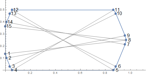
Here is one tile and inner unit distances. All small-scale quantities are increased 10 times.
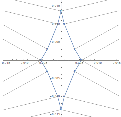
Here is a real size picture of diamond.
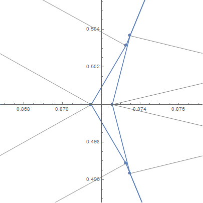
Here is a real size of arrow for convex tiles (6899).
Thanks Jaan!
OK, that is what I was imagining. In the top picture you show 15 vertices, but really the tile has 17 vertices, because vertex 6 includes one at y=d and one at y=d_2, and similarly for vertex 10. Let’s call the ones at d “6a” and the one at d_2 “6b”. I’m claiming that the distance between 6b and the 12-13-14-15 diamond is not optimal, i.e. it is less than 1 from all of them.
Yes, the distance from “6b” to “13” is less than 1. But the tile does not contain the vertex “6b”. This is the vertex from a completely different tile. Just it lies on the edge “6-7”. Therefore, each tile still has 15 vertices. (You can draw an arbitrary number of points on any edge, and finally come to the conclusion that the tile has an infinite number of vertices.)
Ah, I see – there is a problem with our terminologies, because you are considering the diamonds and arrowheads as “gaps” whereas I am considering them as small tiles. But either way, I claim that the tiling can be (very slightly!) improved by making the distance between 13 and 6b equal to exactly 1.
1. I think there are two different ways to define the concept of a vertex. Firstly, as a point at which three or more edges converge, if not a single tile is considered, but a set of connected tiles. In this sense, there is a vertex “6b”, but there is no vertex “6”, as well as “2” and “3”. Secondly, as the break points of the border of the tile. In this case, there is no vertex “6b”. In any case, the number of tile vertices is no more than 15. Yes, this is a problem of terminology. I don’t know how to get around it.
2. And I bet that you worsen the result, not improve it.
In your case, the distance between “6” and “13” will become less than 1, and the area of the arrow will increase.
Right. The only way to get exactly 1 everywhere is with curves. I have nearly completed my construction and characterisation (it has a few extra “break-point” vertices in addition to yours). Stand by!
I look forward to it.
From definition of polygon:
“The segments of a polygonal circuit are called its edges or sides, and the points where two edges meet are the polygon’s vertices or corners.”
I suggest to use words “sides” and “corners” for description of a single tile, and leave the concepts “edges” and “vertices” for the tiling as a whole, where the vertex is the point at which three or more edges meet.
OK, finally I offer the following definition and calculation of what I think (though I do not remotely claim to have proven) may be the truly optimal optimisation of the celebrated Pritikin tiling (which, let us not forget, was originally conceived by Ed Pegg, as reported in the Soifer book). The summary result is that I believe that the best construction is exactly Jaan’s but with d=d_2, so the arrowheads have no corners other than their vertices. He is correct (and it makes sense) that d=d_2 is not optimal if we do not curve any edges (I get 6985.23468, to be precise, relative to Jaan’s 6985.43). However, I am correct that it is optimal if we do curve edges: my final number is 6992.16555 as against Jaan’s 6992.06. My coordinates, using the labels in Jaan’s picture, are:
1 = (0,0.013343547466)
2 = (0.00082693666926,0.0099987220231)
3 = (0.0035745404852,0.0033448254424)
4 = (0.0054885276613,0)
8 = (0.97159339411,1/4)
9 = (0.97076645743,1/4 + 0.0033448254584)
10 = (0.87342791863,1/2 – 0.0033448254584)
11 = (0.87151393145,1/2)
I’ll put the gory details, which involved introducing ten more parameters that all collapsed in the best case, into a separate post.
OK, here goes with the gory details…
First, terminology (which, as already noted by both Jaan and me, can be confusing for tilings). I think the best option is to avoid using the terms “vertex” and “edge” at all.Instead, I will always use the term “junction” to denote points where three (or more, but that’s not relevant for this tiling) tiles meet. Following Jaan’s suggestion I will use the term “corner” to denote points on the boundary between exactly two tiles at which that boundary has zero radius of curvature, i.e. the gradient changes discontinuously. I will also need to refer to a third type of point: one at which the gradient of the boundary does not change discontinuously but the radius of curvature does. I will call this a “quasi-corner”. All boundaries will consist of segments with constant radius of curvature (we won’t have any spirals, in other words), so a quasi-corner is simply a point at which a boundary’s radius of curvature changes between two different (non-zero) values.
OK, here goes. Broadly, the system is as shown in the first of Jaan’s three pictures of today, so I will use his numbering of the junctions and corners. Note that I will use “6” and “10” to denote the junctions at the trailing tips of arrowheads, so “6b” in the terminology of my previous post. My system has all the same diameters (pairs of junctions exactly 1 apart) as Jaan’s, except that I am making junction 13 exactly 1 from 6b rather than from 6a. Note that in my earlier construction a few days ago, I unnecessarily required some extra inter-junction distances to be exactly 1, namely 4-10, 1-9, 15-7 and 12-8 (and their reflections in y=1/4, obviously). This lost me quite a lot, so please don’t try to compare the present construction with that.
The essence of the construction is to incorporate corners and quasi-corners into the short boundaries (i.e. those that are parts of the perimeter of either diamonds or arrowheads) so as to make the big tiles have a diameter of exactly 1 in all directions, except for four angular intervals: between 4-11 and 5-12, between 1-8 and 15-8, between 2-9 and 3-10 and between 13-6 and 14-7. There is nothing new to say about 4-11 to 5-12 or 1-8 to 15-8. The other two intervals are the diagonal directions in which same-coloured big tiles come within 1 of each other: I will call them the inter-tile directions.
In the inter-tile directions, we are interested in distances between counterparts in other tiles of vertices 2 and 3 (and 13 and 14, of course). Specifically, denote the reflections of 2 and 3 in the origin as 2′ and 3′ respectively, and denote the translations of 2 and 3 vertically by a distance of 3/4 and horizontally by the sum of the x-coordinates of 6 and 7 as 2″ and 3″ respectively. These four vertices form a parallelogram 2’3’2″3″, where 2’3″ and 3’2″ are exactly 2 and 2’2″ and 3’3″ are at least 2. It remains to ensure that no pair of points anywhere else on the boundaries 2’3′ and 2″3″ are less than 2 apart. If 2’3’2″3″ is a rectangle, the 2-3 boundary (for any version of 2 and 3) can just be straight, and we’re done.
Otherwise, in order to maintain a distance of exactly 2 in all the directions between 2’2″ and 3’3″, it’s more complicated, but it’s still perfectly possible. I’ll assume 2’2″ is less than 3’3″ (the construction is exactly analogous if we make the opposite assumption). We identify points X’ and X”, located so that X’2″ and 2’X” are exactly 2 and X’X” = 2’2″; thus, X’2’X”2″ is a rectangle. Then we draw 2’X’ and 2″X” as straight lines and 3’X’ and 3″X” as arcs of radius 2 centred at 2″ and 2′ respectively; thus, X’ and X” are quasi-corners. This suffices to keep all same-coloured tiles 1 apart, so long as the (hitherto straight) boundary 9-10 is replaced by a sequence 9-A-B-C-D-10 in which 9-A, B-C and D-10 are straight lines and A-B and C-D are arcs of radius 1 centred on 2′ and 2″ respectively (thus making B and C quasi-corners). A and D need to be far enough around their respective arcs so that 9-A and D-10 do not intersect the unit circles around 3″ and 3′ respectively, but that’s all. BC is parallel to 2’X and 2″X” (and midway between them).
Now for the other angular intervals. We have two quadrilaterals of interest: 3-4-10-11, and 1-2-8-9. (Also 14-15-7-8 and 13-12-6-5, which are the same.) Here the situation is more complicated than the case just examined, because we do not need the short edges of the quadrilateral to be parallel. Our goal is to bend those boundaries so as to optimise the tiling, which involves making the arrowheads and diamonds concave.
As Jaan noted earlier, the best way to do this can potentially involve boundaries with radius of curvature less than 1. My construction (which I have not proven to be optimal, but I think it must be very close) is as follows:
1) The construction is the same for both quadrilaterals, so let’s just consider a quadrilateral ABCD, with AB and CD being the short edges that we’re going to bend. We know that its diagonals (AC and BD) are exactly 1 and AD and BC are at most 1.
2) First we consider the case where AD=BC, i.e. AB and CD are parallel and ABCD is an isosceles trapezium. Here the construction is easy: we replace AB with an arc of radius AB/(AB+CD) and we replace CD with an arc of radius CD/(AB+CD). It’s easy to see that this keeps the diameter to 1, because the maximum distance between the arcs AB and CD in any direction is always a line that passes through the intersection between AC and BD (call that point E), which is simply a rotation of AE plus a rotation of EC. I haven’t proved that this maximises the area of ABCD, but I’m pretty sure it does.
3) Now consider AD!=BC, i.e. AB and CD are not parallel. Let’s assume, wlog, that BC is longer than AD. We now choose a point P such that PC = 1 and PD that is at least AD and at most BC. Then we identify the point Q such that BQ = 1 and PQ = BC. This means that PBCQ is an isosceles trapezium whose diagonals are both 1, and APBCQD is a convex hexagon. We now draw AP and QD as arcs of radius 1 (centred on C and B respectively) and PB and CQ are arcs of radius PB/(PB+CQ) and CQ/(PB+CQ) as in the previous case. Thus, P and Q are quasi-corners. Again it’s easy to see that the diameter is 1 in all directions between AC and BD. But the point here is that we have a new degree of freedom, because of the range of locations we can choose for P.
So when we compare this structure to Jaan’s, basically I an introducing three additional points to optimise, namely the quasi-corners between vertices 1 and 2, 3 and 4 and 8 and 9. The one between 10 and 11 basically substitutes for Jaan’s point at y = w-d.
OK… results. We now have 21 variables (not including Jaan’s “w”, which is clearly fixed to be 1/2), so perhaps it’s not surprising that Mathematica struggles. But I obtained reliable behaviour once I looked individually at each of the 27 cases (three pairs of lengths that can each be either equal or ranked either way). Aaaand, it turns out that ALL the quasi-corners collapse in the best case. In other words, in the best case all our quadrilaterals of interest are rectangles with diagonals exactly 1 (except for 2’3’2″3″, which is a rectangle with long sides exactly 2). Bit of an anticlimax… but I guess it was worth doing.
So. This is a lot of work. But so far I have not fully understood what we have come to (correct me where I am wrong).
1) You introduced many additional degrees of freedom compared to the original 15-gon, but in the end you had to return to this good old 15-gon. At the same time, you came to a result that is more by 0.1, and now we need to understand what causes this difference.
2) If I understand your 2X3 construction correctly, you want to make the X3 arc concave. In this case, the distance 2’3 ” will be strictly less than 2. Is this so?
Last night I sat with a sheet of paper and I got another crazy idea that might work. But today I will not have the opportunity to test it.
Thanks.
1) Yes, we should try to understand the difference. I optimised with curved edges directly. Did you optimise with straight edges and then add the slivers? When I do that wiith d=d_2 I get 6985.37757 and 6992.0266, and I’m betting that with d != d_2 one can get a little more (for both).
2) The hexagon 2’X’3’2″x”3″ is convex. The edges 3’X’ and 3″X” are arcs of radius 2, so they make the diamond concave at that boundary. The other edges are all straight. The distance 2’3″ is exactly 2. The overall hexagon consists of a central rectangle 2’X’2″X” plus two sectors of radius 2.
1) Yes, I thought the same thing. Everything as you described. And this is probably the case. But one need to check everything. A lot of different (close but not matching) estimates have accumulated. For example, I get about 6885.43 for both d = d_2 and d!=d_2, the difference is only 0.004 and this differs from your estimate. And not only this.
2) That’s OK. I drew a little wrong picture.
6985.43, of course
So. Before I did a very sloppy calculation. Some things were supposed, but not checked. And you will laugh, but I just figured out how to display the result with higher resolution. Now we have the following:
1) I repeated your result 6985.2346760 and 6992.1655504 for the case of joint optimization of the 15-gon and the curving segments of the short sides of the tile.
2) I got a slightly different, but close, result for separate optimization: 6985.3775668 and 6992.026378 (my) vs. 6985.37757 and 6992.266 (yours). Moreover, if we do not assume further curving of the short sides of the tile, then we can get 6985.429624 for d!=d_2 and 6985.426227 for d=d_2. In this case, the curving radius cannot be less than 1 and after curving we get 6988.746463 for d!=d_2.
3) My new idea is somewhat similar to yours. It consists in the fact that we can free the common point of the opposite sectors of the circle and allow the sectors to be slightly inclined, not strictly opposite. Further, the sectors in each pair can have different radii (the sum of the radii is 1). Verification showed that this does not provide improvement.
4) One can continue the generalization further and allow for each direction on the plane its own radius. As a result, we obtain a continuous dependence of the radius on the direction. This is an infinite number of degrees of freedom. Then one can try to optimize this function. I do not know if this can give anything. Based on the results already obtained, there is reason for doubt.
Correction: 6992.026378 (my) vs. 6992.0266 (yours)
Great. Concerning (4), yes, that is what I meant when I referred to spirals, and I agree that it is unlikely to help, though I don’t immediately see a way to prove that the construction using only sectors and fattened isosceles trapezia is optimal.
Shall we move on to the 5-tile pattern?
Yes, we will do it. But first, I need to prepare a good start. This task looks much more complicated than the case of 5 colors. And this is a nightmare, how much time we spent on an elementary case of 6 colors. Therefore, I want to start with a picture and distinct designations. And with a good initial solution. But this is not ready yet.
Damn, 6, not 5, but you got it.
I’m hoping that some of the principles we learned last week will translate to the 5-colour case… but yes, it is really daunting.
Right guys, I am feeling a bit better now about spending so long last week on optimising Pritikin, because the ideas involved have led me to a really nice result. We were talking recently about 7-tiling an arbitrarily large sphere, but we also have the question of how large a sphere can be k-tiled for smaller k, for which the current results are the ultra-boring tetrahedron, square pyramid and dodecahedron. I’ve just realised that Philip’s 6-disc can be used for each face of a dodecahedron, giving a 312-tile tiling of a shere of diameter, um, quite big. Here are a picture of a region, and the details.
First we note that Philip’s disc can be extended quite a lot with the addition of 10 very small tiles of a seventh colour. (Interestingly, they can all be one colour: they come in Siamese pairs.) They are the small dark-shaded triangles denoted 7a, 7b, 7c in the figure. So here’s where it gets interesting. If we ask what colours the next ring of tiles can be, we see that the four at the top are analogous to the ones below them: 1,3,4,1 adjoins 6,5,2,6. It’s easy to see that this works all the way round. So now, suppose we take a dodecahedron and replace a face with a 6-disc. Then, the neighbouring faces of the dodecahedron can also be replaced by 6-discs, and everything works – the midpoint of each edge of the dodecahedron has four tiles meeting that are the colours not used for the centres of the dodecahedron-faces that meet at that edge, and the symmetry of the original 6-tiling does the rest.
So it remains only to determine that the colour-7 tiles vanish when we do this. That’s easy to see, because (in the plane) those tiles are entirely above the line (in the plane) between two adjacent tips of the 6-discs, which equivalently means it would be entirely above those small tiles if we were considering the adjoining 6-disc with central tile coloured 1. (I hope that makes sense!)
So the radius of the sphere is, um, I think something around 4. Can someone come up with an exact formula?
Also, can we use our 5-discs to get a better result for a 5-sphere?
Also also, obviously pentagons can’t be used to tile the plane, but can we fill in the gaps with large tiles not using colour 7, i.e. can this design be the basis of a tiling of the plane that beats Pritikin? I’m not sure what the area of the small tiles is, but I suspect it is small enough. A dense tiling of the plane with pentagons allows each pentagon to share three edges with other pentagons, and we just noted that small tiles at shared edges go away, so effectively each pentagon has only four small tiles rather than ten. I have run out of time for today but I’ll look more at this soon.
Peter’s new result claims that 8 colors are needed if the radius is at least 18, but there are some unverified calculations in it right now.
Oh, and that is only for the more restricted case of ‘scalable’ tilings that Thomassen considered.
If anyone is interested, here is my (hopefully essentially correct) proof:
https://drive.google.com/file/d/1Q8QYljpIgAOPr8kxVS6uIsAGEH4Z97S9/view?usp=sharing
I have spent quite a long time trying to obtain colourings with 8 (or at least with 9 or 10) colours for all large enough spheres, but I haven’t succeeded yet, so the best colouring I know of that does not only work for spheres of bounded radius is still 15, which follows from the colouring of the 3-dimensional space.
I was also interested in the proof of the tiling-based chromatic number of the plane being at least 6 (so I could possibly use it for constructing a similar proof for spheres in the general tiling case (as Dömötör wrote, I was only considering the “nice” tilings considered by Thomassen)), but sadly the Townsend paper isn’t openly accessible as far as I know (it has been published in Geombinatorics), while the one by Coulson (that is also listed in the wiki as a proof for ) only considers convex polygonal tiles (unless I completely misunderstood something).
Many thanks Peter – wow, this looks very impressive – I will study it thoroughly when I have more time. I can email you the Townsend paper if you email me at aubrey@sens.org.
Meanwhile, I was so astonished by your finding that large spheres are hard to tile even with more than eight colours that I had a go. I believe I have a tiling with 11 colours, using the classic “geodesic dome” tiling with 12 pentagons and a lot of hexagons; I don’t think the variation in size of tiles arising from the curvature is enough to make problems, but please shout if you think it does.
Let the tiling be such that there are 3n+1 hexagons in a chain between each pair of pentagons. Assign each of colours 1 through 6 to two opposite pentagons. Then assign each of 7 though 11 to the chains of hexagons joining pairs of pentagons, i.e. to edges of the mega-icosahedron; say we use colour x for a chain between pentagons of colours y and z, we colour the hexagons x,z,y,x,z…y,x. Assign each colour to six edges such that each vertex uses each edge-colour once; the midpoints of edges with the same colour end up being at the vertices of an octahedron. Then consider the hexagons within a face of the mega-icosahedron, i.e. the triangular grid of hexagons that is bounded by three inter-pentagon chains. 2/3 (or so) of these hexagons are a multiple of three hexagons away from some hexagon on an inter-pentagon chain; assign them to the same colour as that chain-hexagon. (In some cases two such chain-hexagons identify the same face-hexagon, but they are the same colour so there’s no problem.) The remaining hexagons in the triangle can then be coloured using the three vertex-colours not used by the pentagons at the triangle’s vertices. This seems to create no conflicts in the neighbourhood of vertices or chains.
Here’s a quick ASCII-picture, with n=3, centred on a pentagon of colour 1 that I have denoted with a *, and the edge-colours are t,u,v,x,y. Note that this is the whole of the five faces of the mega-icosahedron – the 120 degrees between 7 o’clock and 11 o’clock is just one such face, stretched vertically, so as to allow the other four faces to be shown as equilateral triangles. Thus, all five corners of the grid shown are pentagons.
Please let me know if I have hereby redeemed myself after yesterday’s debacle!
Heh, looks like posts go to moderation purgatory even with just one hyperlink, if they also contain an email address…
Thanks Aubrey, I sent you an e-mail about the Townsend paper.
I also had quite a few tries on making colourings based on dividing an icosahedron (or even an octahedron) to tiles, and apply a colouring in which no two neighbours or second neighbours have the same colour, and some of them seemed to work (my primary goal was to find an 8-colouring, so I did not try giving colourings with much more colours for a very long time):
For example below you can find a 10-colouring of an icosahedron (I am not fully sure it is correct, I might have overlooked something in it (the tiles near the borders of the net were made in an ad hoc manner, which makes it much harder to check the correctness), but I think it can be generalized by dividing the colouring to clusters around the blue tiles and if we take a larger icosahedron, we can simply copy the clusters along the borders of the net, while those in the interior will be coloured with an Isbell colouring as they are in this colouring).
You can also find a 9-colouring of an octahedron (it can be generalized much easier as it is much more regular), I have also tried to make similar colourings for icosahedrons.
https://drive.google.com/open?id=1YsP8wd5h8pFkfjLsd6eOZuGdTJ-SA3-m
But sadly it seems to me, that simply projecting such colourings from an icosahedron to a sphere from their common center causes more distortion in the colouring as one would think (not to mention octahedrons):
The circumradius of an icosahedron of edge length 1 is , so if we name its center O, one of its vertices A and the midpoint of a face having A as a vertex M, then
  meaning that for any sufficiently small segment sufficiently close to M, projecting it to the circumscribed sphere will scale its length by a factor sufficiently close to
  . Also, if we take a sufficiently small segment starting from A, the projection to the circumsphere is almost like an orthogonal projection, so its length will be scaled by a factor sufficiently close to
  . So in total the ratio between the images of two segments of the same length can be arbitrarily close to
 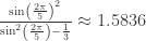 . And even though Isbell’s colouring is scalable, the ratio of the distance of two tiles of the same colour and the diameter of a tile is
  . So here even if all pairs of tiles of the same colour have graph distance at least 3 in their adjacency graph, it is not necessarily enough for a large enough sphere (it depends on how those with graph distance 3 are located).
(Side note: Dömötör also told me a few times while I was working on the proof for the Thomassen type chromatic number of the spheres being at least 8 that it might be easier to only look at a large enough disk in which no tiles with 5 neighbours occur and get a contradiction from that, and the above means that he might have been right.)
Of course the above does not mean that by using some trickier projection, one could not make a good colouring on spheres.
The good news is that it seems that in your colouring, pairs of tiles of surface distance only occur such a way that the two tiles are separated by an edge of the icosahedron, so even if it is not good for spheres (I haven’t calculated it yet), it is possible that some modification around the edges (like replacing the edges with very long, narrow rectangular faces and the vertices with small pentagons) resolves the situation. Anyhow, it needs a bit more calculation, but it is completely possible that based on your colouring all large enough spheres can also be coloured.
Thanks so much Peter! Very nice colourings.
I’m confused by your scaling calculation, though. The way I did it was just to look at the ratio of the radii of an icosahedron’s circumscribed sphere (which is sin(2*pi/4) as you say) and its inscribed sphere, which is (Sqrt[3]/12)*(3+Sqrt[5]). The ratio of these two numbers is 1.258, which is less than the scaleability factor of the Isbell tiling. The value that you get seems to be the square of this – and indeed, you seem to be expanding the tiles near M but also shrinking the ones near A. What am I not understanding?
Yes, exactly. All segments near M go to nearly parallel segments after projection, and they are scaled with 1.258… compared to their original length, because as you wrote, that is the ratio of the circumradius and the inradius (I wrote it in a bit more complicated way, but we are talking about the same thing). But also, those near A, which are directed towards M go into segments roughly at the same place, but their direction is not parallel with the original one, thus they shrink with the same ratio as with what the other ones were expanded:
If we take such a segment AP, then its image will be a segment AP’, where tends to $90^{\circ}-\angle{MAO}=\angle{AOM}$ if P tends to A. The projection that takes AP to AP’ is almost an orthogonal projection (it tends to it if P tends to A), so the ratio of the projection tends to
  if P tends to A.
So in total the ratio of the two images is the square of 1.258… (unless I am overlooking something).
Ah, I see, you’re taking into account that the tiles near the icosahedron’s vertices are inclined relative to the circumscribed sphere, so they will shrink when you project them onto the sphere. Fair enough. But I’m pretty sure it’s OK, because of the specifics of which same-coloured pairs of tiles are at the Isbell distance – namely, they are juxtaposed almost perpendicular to icosahedron edges, so the shrinking will not significantly reduce their separation. Right?
[reposting in the right place!]
Ha, we posted at the same moment. Yes, thank you. The hexagons near to the pentagons must clearly be somewhat distorted anyway. But maybe it still doesn’t work? I don’t have a rigorous mentalimage of this yet.
Me neither. It needs a bit of more calculation to tell if it works or not. But as I already wrote, if it doesn’t, it is still possible to replace the edges with long, narrow rectangles, but it makes the calculation even uglier.
OK, I now feel convinced that the difficulties arising from the stretching and shrinking that arises from projecting onto the sphere can be resolved simply. We consider each face of the un-sphericalised mega-ico separtely; a face is tiled with a standard honeycomb of congruent hexagons, with half-hexagons along the edges and a kite at each corner. Suppose that there are N half-hexagons along an edge. First, we define a diameter d for the hexagons, and a number x around 1/3 (let’s just say 1/pi), and we identify the six points on the edges that are dNx from a vertex. We then draw lines from each of those points, perpendicular to the edge on which they appear, so as to divide the face into seven regions, namely a central triangle, three rectangles and three kites at the corners. Then we do the same thing with a different value x’ that is just a little bit more than x, call it x(1+y). We then map all the vertices of our tiling according to y – in othe words we expand the kites uniformly by a factor x’/x, we shrink the central triangle by a factor (1-2x)/(1-2x’), and we change the aspect ratio of the rectangles accordingly. Finally we project this deformed grid onto the sphere. After some rough calculations, I’m pretty sure that there is a respectable range of values for d and y that makes every Isbell pair (including those that cross between regions or between faces) further apart than any hexagons diameter.
Yes, I also think this will work (if I understand it correctly, this is a different formulation of the same colouring I recommended by replacing the edges with long, narrow rectangles (it uses a different polyhedron, but results in the same colouring after projection), but your formulation may be better for the calculations).
I was considering such modifications, while making colourings (and other modifications of the shapes of tiles near the border), but I could not obtain an icosahedron colouring which only contains bad pairs on different faces, so I didn’t do the exact calculation.
Wow. But I do not believe it yet. Let’s turn to the picture. Apparently, the edge (or side) between tile 1 from the bottom row 34134 and, say, adjacent tile 5 should give a straight line, since this tile 5 has a common vertex (or corner) with tile 1 from an neighbouring face of the dodecahedron. And this is possible only when the radius of the ball is the same as that of square pyramid. Or I’m wrong?
Thanks Jaan for having a look. No, it’s OK. In the plane, the rigid diagonals of the tiles coloured 1 and 5 go between a {1,5,4} junction (call it A) and a {1,3,5,6} junction (at 2 o’clock on the central tile of the main disc; call it B) and between A and a {1,5,7} junction (call it C) respectively. As you say, there would be a “fattening conflict” at the 1-5 tile boundary if tile 7 did not exist, because the angle made by those diagonals is slightly less than 180 degrees. But the curvature of the sphere fixes that: the circle with its centre at the centre of the sphere that passes through B and C also passes through A, i.e. that angle is now exactly 180 degrees, so there is no fattening conflict any more. This happens because viewed from the centre of the disc, A is slightly clockwise of C, even though viewed from B it is slightly anticlockwise.
I do not understand yet. Let me clarify. We consider the sphere and coloring in 6 colors after the disappearance of small tiles (with color 7). We continue to denote the junctions: {1,5,4} – A, {1,3,5,6} – B, {1,5,2} – D, {1,3,5,6} – E, and {A, D, E} are the corners of tile 1 from the bottom row of the picture, {A, B, D} are the corners of tile 5 from the adjacent row above. Tiles 1 and 5 share a common AD side. Both junctions B and E connect tiles with colors 1 and 5. As a result, we get a chain of colors 5-1-5-1 (from bottom to top, from right to left). Is it right so far?
My E is your B (sorry)
Yes, that’s all correct.
Ha, we posted at the same moment. Yes, thank you. The hexagons near to the pentagons must clearly be somewhat distorted anyway. But maybe it still doesn’t work? I don’t have a rigorous mentalimage of this yet.
Good. We continue with my notation. We have a rhombus with sides AB, BD, EA, ED, which are all equal to 1. And we have a side AD, all points of which must also be at a distance of 1 from points B and E. So?
Ahhhh… now I understand your challenge – I had not looked at the 1,2,5 junction. Hm… I need to think about this, but it does seem to invalidate the construction as I described it so far. Thanks!
Yes, I think that this is possible only when large circumference of the sphere (or how is it called?) has length 4. That is, when the radius of the sphere is (2/pi).
Correction of terminology. I thought (apparently wrong), that you meant half-sphere naming it squared pyramid. In this case the whole sphere is octahedron, of course.
I suggest to think about whether it is possible to wind many layers of your 312-tile dodecahedron onto a sphere of radius (2/pi)? Or are there even more problems with self-intersections? But it could be an interesting multi-layer sphere (instead of boring octahedron), if you’re lucky.
Funny question: what is the minimum number of colors required for proper coloring of “6992”-tiling (including diamonds and arrows)? Looks like 9 colors is enough. Who finds less?
I think nine is correct. Reciprocal question: what is the largest number you can get while still only using seven colours, i.e. by stretching the tiling vertically and compressing it horizontally so that the small tiles can all be the same colour? (Clearly it must not have any arrowheads, only diamonds.)
Hey, it was my question.
I’m doing it now. And again faced with the instability of the solution while maximizing. I’m trying to understand which system of constraints leads to a quick and stable result. The same problem appears in the case of 5 colors, so we need to understand simpler examples. I decided to start from the very beginning and gradually increase the complexity of the tiles. Here are the current results so you can check them out.
1. Classic 7-gon of Pritikin: 5681.489884345 for 7 colors (vs. 302.0962 by Edward Pegg), 6197.579308329 for 8 colors.
2. Pritikin’s 7-gon with wavy inclined sides (11-gon in fact): 5782.990890412 for 7 colors, 6295.897444136 for 8 colors (with side-2-rectangle constraint I get more stable solution, but only 5780.207842396 and 6294.390840579).
Great work Jaan! I had not actually noticed that Pegg’s original design allowed the small tiles to be all the same colour – we must mention that in the paper.
Ah, but I don’t understand the last pair of numbers. What is the difference between “with side-2-rectangle constraint” and “classic 7-gon of Pritikin”? In my understanding, they are the same thing.
There is a difference. But let me explain this a bit later. By the way, the parameter w was introduced (a long time ago) precisely for 7 colors task. And I have not finished. There will be options with a 12-sided diamond and curving.
So far, a stable solution is obtained for a 9-gon with wavy inclined sides (13-gon in fact), but here I must also check these wavy sides. Diamond has 8 corners. There are problems with the 12-corner diamond. It seems like I know why: the functions of sides of diamonds are changing. For a non-curved 9-gon, I got 5976.095681162, after curving of some short sides 5977.261894810.
Now about the terminology. I call a classic 7-gon the one without curving and without wavy sides, that is, an usual 7-gon with straight sides. Next, I examined a 7-gon with curved inclined sides and the usual 4-corner diamonds. There are options on how to set a distance of length 2: the sides of diamonds can form a rectangle, or a parallelogram. After that I tried to increase the number of corners of diamonds.
I will continue further.
Correction: …examined a 7-gon with wavy inclined sides…
I played with a 12-gonal diamond a little more. It looks like it is collapsing into an 8-gonal diamond. So the best solution that I get for 7 colors so far is 5977.261894810. Aubrey, could you confirm this result?
I also think that the cause of the unstable solution is the appearance of vanishingly small quantities that lead to degeneration of matrices and division by 0 in the process of optimization. But so far I can’t solve this problem.
Tell me exactly the constraints on your tiling and I’ll check it.
While I was preparing a detailed answer, (it seems) I’ve found the reason for the poor convergence of the solution. I was let down by my generosity. I used constraints of the form =4 between all possible corners, in addition I used similar constraints between all points and line segments. It turned out that if I leave only constraints of the form ==1 and ==4, then this improves the convergence of the solution by several orders of magnitude.
I propose the following notation. We take the original image of the 15-gon given earlier. In the case of 7 colors, the pairs of corners 8–9 and 10–11 are collapsed into two corners. I don’t want to use other notations, so I just drop the corners 9 and 10, and leave 8 and 11. To work with constraints of length 2, we need to mark the tiles of the diagonal row around two neighbor diamonds. Let it be tiles a, b, c, d (from left to right, from bottom to top), with b being the base tile (drawn earlier), a – its reflection relative to the origin, d – the tile shifted by (g+h, 1.5w) relative to the base tile b. Then the necessary points of the plane are denoted by a pair of letter-number.
For 7 colors with reduced set of constraints {| b1-b8 |==1, | b2-b8 |==1, | b3-b11 |==1, | b4-b11 |==1, | d3-a2 |== 2, | d2-a3 |== 2, | d2-a2 |==| d3-a3 |} the result is 6043.112467879 (if I was not mistaken somewhere).
Yeah, latex ate part of the text. It was written …used constraints of the form “equal or less than 1” and “equal or more than 4″…
Um, you also need 2*|b4 – b12| == |b1 – b15| + 1, right? Please confirm before I get on this.
Sorry, I of course meant |b4 – b12| + |b1 – b15| == 1
Yes, in other notation it is (w-a)==1/2.
Hm, I’m not reproducing it. I’m getting a maximum of 5874.62, with points 1..4,8,11 being at (0,0.0142901), (0.000655472,0.0116867), (0.00398441,0.00390976), (0.00631691,0), (0.970063,1/4+a/2) and (0.863933,1/2+a). My central parallelogram does not collapse, though it is a rectangle (the parallelogram is slightly smaller but the gain is outweighed by the radius-2 slivers). What are your coordinates?
Thanks, Aubrey. I am not surprised. Whenever I run optimization, I get a new result. It is like a random number generator. Our results may coincide accidentally, but we will never know the right one.
I substituted your values and got 6042.52977236409. But some distances are slightly more than 1. I also got almost your 5874.63162557873, if instead of w, I use 0.5 when calculating the total area.
Hm, I’m not having any such problems with reproducibility. Also, I’m checking the lengths of diagonals arising from the returned values and they are all coming out exactly right (well, to within 10^-15). I think you must have a bug somewhere.
Ah, damn, I maligned you! I was the one with the bug – I was indeed calculating the number using w=1/2. I now obtain 6043.112468 with (0,0.0143908), (0.000721488,0.0115263), (0.00400433,0.00385627), (0.00630569,0), (0.970075,1/4+a/2), (0.863862,1/2+a).
Ten out of ten digits match. It’s a miracle.
I guess now is the time to switch our attention to five colours. I’m simultaneously pursuing several other strands of the paper, as you can see, but I’ll try to do something.
Something we must not forget in the paper: I just realised that the slanted edge 9-10 in Jaan’s picture is not precisely parallel to the edge 2-3 – the slopes are about 2.4996 and 2.4217 respectively (this is for the standard 6992 case). This means that there needs to be a zigzag in the middle of the 9-10 edge, so that the central section is exactly parallel to 2-3. So our large tiles get four extra vertices.
In fact, it’s enough to add two corners to each tile, if you keep in mind that you can slightly extend the side 8-9. As a result, the tiles will be 17-gonal. (I’m getting greedy.)
Ah yes, that’s neat!
Meanwhile I thought I would have a look at reducing the number of parameters for the tiling, so as to be able to describe it more concisely. If we hard-wire the assumption that 1-2-8-9, 2-3-2′-3′ and 3-4-10-11 are all rectangles, we end up with a system of six equations in seven variables, which can very straightforwardly be reduced to a single equation in two variables, namely the y-coordinates of points 1 and 3 (call these y1 and y3), with the other coordinates all being simple functions (well, at worst the sum of three square roots of quadratic expressions) of y1 and y3. That remaining equation, however, contains four different square-root expressions, and takes some work to transform into a polynomial; in the end I obtain an octic equation in y3, whose coefficients are polynomials of degree up to 14 in y1 some of whose numerical coefficients are in the trillions. Somehow I think we can omit the details from the paper :-).
Does anybody here have this paper:
Croft, H.T.: Incidence incidents. Eureka 30, 22–26 (1967)
I have circulated a draft note by email on upper bounds in higher dimensions. This note can be included in a polymath paper. The results have appeared in earlier threads and are in the wiki.
Aubrey asked some general questions so I will post some partial answers here to keep it open.
We found new upper bounds for 5 and 6 dimensions using permutohedron tesselations and linear colourings, adding to previous published bounds in 2, 3, and 4 dimensions. For up to 5 dimensions the search is exhaustive so we know these are the best bounds of this (very restricted) type
A permutohedron in n-dimensions is an n-dimensional polytope formed from vertices whose coordinates in n+1 dimensions are the permutations of the first n+1 positive integers. The minimum width of the permutohedron is and its diameter is
  . If it is rescaled to have unit diameter then the minimum width is
  . At n=10 this is 1/2
We need to find all “dangerous” cells that have points within unit distance of a central cell in the tesselation. For from 2 and 10 dimensions this will be the touching cells and the next layer out that touches those cells. There should be a formula for the the number of cells in these layers which we can find to give us the number of dangerous cells up to n=10. For n >= 11 some additional cells from the next layer must be included but this is well beyond where we can currently search anyway.
Thanks Philip! You already corrected yourself in email regarding the third layer, so let me just save others the trouble of pointing out that we get third-layer cells in the danger set even as soon as n=4.
I have coded up the geodesic dome as a graph with the faces as vertices and edges between faces that share a boundary or that both share a boundary with the same third face, and I’m throwing it at my Mathematica SAT solver for increasing numbers of hexagons between pentagons – and the big news is that it’s very rapidly returning SAT for 9 colours for every length (though it’s getting pretty slow by now at building the graphs and clauses). I’m not checking 8 colours yet because that already got really slow even for n=3 (it is SAT for n=1 and 2); I’ll try that overnight. I’m up to n=16 so far, i.e. comfortably into Peter’s radius-18 territory. (Reassuringly, it’s always returning UNSAT for 7 colours.)
Turning this into a colouring for arbitrary size may be hard, though… if I get time I’ll have a look at the small cases and see if I can discern any pattern, but the speed with which solutions are being found leads me to fear that there will be a lot of randomness and nothing will leap out without massive serendipity. If I get an 8-colouring for n=3, I’m hoping things may be better in that regard, since evidently if such colourings do exist they are rare.
Note that I am only looking at the simple case where there is a straight chain of hexagons between edges; I have not explored the skewed cases such as the one Peter shows on his Google Drive page. Presumably those are also worth checking wrt 8 colours.
Update: the geodesic sphere with three hexagons between pentagons cannot be 8-coloured. My solver established that in ten minutes; it was undecided on the four-hexagon sphere when I aborted it after two hours.
I’m now asking what happens when we replace each vertex of the mega-ico by a Gibbs disc; this can be done quite efficiently starting from the geodesic graph, by just removing the five vertices (i.e. hexagons) neighbouring each pentagon-vertex and adding 240 new edges (20 for each pentagon). (It only makes sense when the initial geodesic sphere has at least five hexagons in the inter-pentagon chain.) Sadly I am not getting any improvement on the simple geodesic sphere: with n=5 it is hanging for 8 colours. I think there is a good chance of improvement using Peter’s skewed design though (and variants thereof). I’ll try to get to that soon.
That is surprising! I would have guessed that it becomes 8-colorable for very small n. Is it possible that for larger n the program would run faster because it would have more freedom?
Possible, but equally it could go more slowly if at small n it is still truly not 8-colorable. But my intuition is that skewing makes a big difference, allowing Isbell-style colourings to encroach closer to the Gibbs regions.
Philip tells me he has posted something here – Dustin, is it in purgatory? [I found it in the spam folder. -DGM] It is a brief writeup of the work on upper bound in higher dimensions, extending Radoicic and Toth, which will be a sectionin the paper.
Meanwhile I too have been looking at higher-dimension tilings and I’m fairly hopeful of progress. I have been looking at the Weaire–Phelan structure, hereafter WPS (see Wikipedia for details), which was shown to have a fractionally lower surface-to-volume ratio than the permutohedral (“Kelvin”) structure, and which I think has a slightly smaller set of prohibited neighbours (for both types of cell) than the 65 we get for permutohedra, by virtue of the fact that 1/4 of the cells are dodecahedra rather than tetradecahedra. That won’t translate into a tighter upper bound, of course, because the presence of any tetradecahdra limits it to 15. However, I’m more optimistic when we generalise the WPS to higher dimensions. I’m proceeding as follows:
If I’m not mistaken, the WPS tiling of R^3 can be described as the Voronoi tiling arising, for all triplets {i,j,k} of integers, from “type A” points (4i,4j,4k) and (4i+2,4j+2,4k+2), which lie at the centres of the dodecahedra, and “type B” points (4i,4j+2,2k+1), (2i+1,4j,4k+2) and (4i+2,2j+1,4k), which lie at the centres of the tetradecahedra. For our purposes the key degree of freedom is that the planes separating type-A cells from type-B cells need not be exactly midway between their respective points: we can choose how far along the AB line they sit, i.e. shrink or grow the type-A cells, so as to make both types have the same diameter. (I think the fact that B cells necessarily have a width of 2 makes this optimal.)
I think the best generalisation of this to R^n is to have type A points be those with all coordinates 0 mod 4 or all coordinates 2 mod 4, and, for all i in 1..n, to have the type B points be those at 0 mod 4 for dimension i mod n, 2 mod 4 for dimension i+1 mod n, and 1 mod 2 for all other dimensions. This seems to give type B cells a width of 2 for any n, and type A cells a width of Sqrt[n+2]. Where it gets interesting is with the diameters. I think type A cells have a diameter that is an at most logarithmically-increasing (or even bounded?) multiple of Sqrt[n+2], because each type A cell has a pretty dense packing of B cells around it. But this also applies to type B cells – I think their diameter is bounded at slightly more than Sqrt[10], or at worst rises logarithmically in n. (There are n times as many type B cells as type A, so maybe it isn’t crazy that the dimensions of type B would grow more slowly? Or is this offset by their constant width?) This would mean that when we shrink the type A cells to make the diameters equal, we shrink them more for higher n – in other words, we end up with a diameter/width increasing more slowly than O(Sqrt[n]), which would surely translate into a better chromatic number than for permutohedra. But I haven’t fully convinced myself of all this yet – all help welcome.
No luck yet with skewing… but I have noticed that there’s a conflict (just one, it seems) in Peter’s attempt at a 10-tiling of a skewed icosahedron:
I’ll try to get Mathematica to render some 9-colourings soon.
Actually there were several more (including two neighbouring red hexagons that are visible on your screenshot). I hope I have corrected the colouring now:
https://drive.google.com/drive/folders/1YsP8wd5h8pFkfjLsd6eOZuGdTJ-SA3-m?usp=sharing
Looks good! Meanwhile I have figured out an elegant way to encode skewing, so I will try a few more things today. I will also export the clause lists for these graphs so that those with superior SAT solvers can attack CN=8 for the various spheres.
Everyone: the burst of activity stimulated by the plan to write an all-encompassing upper-bounds paper leads me to propose a slight change of plan. I had (more or less) promised Soifer that we would submit in time for his next issue, but it’s now clear that if we were to try to do that the result would be horribly rushed and incomplete. Therefore, I propose that we aim for the following issue, which may allow us to present properly polished discussions of the various outstanding areas (5-proportion, 6-disk, n-sphere, non-permutohedron tilings)as well as the areas where we are already satisfied that we have closure (4-strip, 5-disk, 6-proportion, permutohedra). I will pacify Soifer with a writeup of my 59-vertex 6-chromatic thing in R^3, which was not really part of the Polymath project anyway and which I think I can get done in time for the upcoming issue.
Unless anyone objects today, I will notify Soifer accordingly.
I think we don’t have to pile everything together in one heap. It is much better if there will be a separate article in each direction. I will try to be in time with the “tiling of the maximum fraction of the plane with a limited number of colors”.
Maybe you’re right. Especially if Philip and Tom reach some kind of closure on their attempts to perform an exhaustive search of non-Siamese 6-tilings, that would merit a stand-alone article. I think the new 5-disk and the refinement of the Bock 4-strip are too small, but they would naturally be addable as notes in the 6-tiling article. As for the higher-dimension tilings, I hope to have something to say soon about generalising the WPS and it may end up being substantial enough to merit a stand-alone article, which I don’t think the permutahedron calculations do on their own. That leaves only the sphere, where the main result as of now is the remarkable difficulty of tiling with eight colours (let alone seven), or indeed with nine or ten in a simply-describable manner; I have a feeling we are at only an early stage in that investigation, so it should probably be deferred anyway.
OK, so what does everyone think of the following sequence of papers:
1) me on the 59-vertex thing in R^3, including its generalisation to higher dimensions (which I have just improved, actually)
2) Jaan on fraction of the plane, including both 5 and 6 colours (and the Siamese 7-tiling)
3) Philip and Tom on non-Siamese 6-tilings, with brief notes on the 4-strip and 5-disk
4) me and Philip on higher-dimensional tilings if the WPS idea turns out to be fruitful enough
5) eventually something on spheres
I’m thinking that (2), (3) and maybe (4) could be in the final issue of 2020. There is also a bunch to be written on lower bounds, of course, presumably as a parallel sequence of papers, but I don’t have a good sense of how to attack that – I invite Domotor to suggest a strategy.
Aubrey, please clarify how much time we have left? Or am I definitely not in time for nearest issue? (Now I am preparing a brief report on 5 colors, not enough free time.)
I will ask Soifer today about timing for the two issues. However, I think the 5-proportion work is really eye-catching and should not be rushed; I am sure he would prefer a thorough report in the next-to-next issue rather than a short one in the upcoming issue, and I agree. I am happy to help with it; maybe when you have a brief report you can circulate it and we can work together on the details.
It looks like soon there will be enough articles to fill a whole special issue 🙂 The good thing about that would be that there is no strict deadline then… About the lower bound works, Peter has a nice argument about the chromatic number of the sphere (discussed above), plus we have some partial results about the probabilistic formulation (see the old threads), and then there’s the bichromatic approach (on which I’ve worked with Nora and Tamas a while ago).
Well. Now about tiling the maximum fraction of the plane using 5 colors.
To begin with, I would like to introduce additions to used terminology. When tiled, a part of the plane remains uncolored. In the case of 5 or 6 colors, the uncolored area becomes multiply connected. Each connected uncolored region will be called a void. Each connected colored region will be called a tile.
We will distinguish three types of tile sides: straight, curved and wavy. Each side is bounded by a pair of corners (points). Curved side differs from wavy one in that the former have one single optimal shape, while the latter allow many different optimal shapes.
We restrict ourselves to one specific case of periodic tiling, in which there are 5 types of tiles (indicated by the numbers 1…5). Tiles of each distinct color have a fixed shape. Two pairs of colors (1 and 5, 3 and 4) have tiles of mutually mirror shape, the remaining tile (2) is mirror self-symmetrical, so it’s enough to talk about three types of tiles. Four types of voids (indicated by the letters a…d) are distinguished in a similar way. All types of voids, except b, are mirror symmetric.
When designating points (corners), it is more convenient to snap not to tiles, but to voids. We will number the points of voids clockwise, starting from a specially marked (larger) point with number 1. In the figure (below), we added points that are not corners, but are used in calculations. We are also expanding the range of named voids to make it easier to set distances. Additional voids are obtained from the voids a…d by reflection from the vertical axis and transferring by cell (x, y). One cell contains a minimal repeating tiling element and includes 2.5 tiles and 4 voids. The number of points of voids: a – 12, b – 4, c – 8, d – 16. Points are indicated by a pair of letter-number (the letter indicates the certain void).
We will distinguish 3 types of constraints on tiles: inner with a diagonal length of 1 and outer with a side length of 1 or 2. It is convenient to consider groups of constraints of 4 points. Such a group defines a trapezoid and in the simplest case is described by equating two pairs of sides and diagonals, for example: {|1-2|=|3-4|=1, |1-3|=|2-4|}. In the case of outer constraints, this method is not quite correct, because it allows the opposite sides to be closer (12 and 34). But in our case even such incorrectly defined constraints lead to the correct result (it turns out that |1-2|=|3-4|). That is, all trapezoids become rectangles. This indirectly indicates the stability of the solution. (Other types of constraints were also considered, but they did not provide improvements.)
After I pressed and wrinkled a little described tiling, I got such a result. The reciprocal of the uncolored fraction of the plane is 24.9627819109. I wonder if it is possible to suppress somewhere else to add the missing 0.04? (We need +0.16% only.)
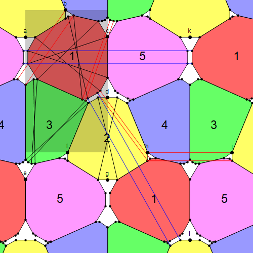
Groups of constraints:
a) inner (shown black): с1c2a4a5, a2a3d8d9, b2b3d5d6, d2d16g2g16, d3d4e5e6, a5a6e7e8
b) outer with side length 1 (red): b1b2a8a7, c6c7d5d4, h3h4d8d7, h1h4j1j4
c) outer with side length 2 (blue): d6d7i3i2, a10a11k4k3
Here is a picture. Curved or wavy sides are shown as straight sides (simpler to draw). (What did I forget to say?)
Jaan, this is so cool. Even with all the rectangles, that’s a lot of variables. I’ll have a look at it in the next few days.
I corrected the picture a bit to show the base cell, including tiles 1…3 and voids a…d. In my case, the variables are the coordinates (not all) of only those points (corners) that fall inside this cell. The remaining points are obtained by translations and reflections.
According to my observations, an increase in the number of variables does not significantly worsen the convergence of the result. This time I started with about 30 variables and brought them to 39, gradually removing restrictions that seemed “natural”, but in fact worsened the result a little. Two reasons that lead to poor results are the wrong choice of the initial approximation and the use of inequalities instead of equalities in constraints.
Here is more detailed picture with curved and wavy sides. All rigid sides shown solid, wavy sides shown dotted (straight line) or dashed (arc with radius 1).
Jaan – a quick request on another topic. Since we will be including (somewhere) a brief addendum to Bock’s paper, correcting the construction and giving an exact value for the width, it would be nice to have a strong upper bound. At present I think the best we have is your construction of a 5-chromatic graph that fits within a strip of width 1.4. Could you modify your program so that instead of being 5-chromatic, the graph only needs to have a vertex pair that is always monochromatic in any 4-colouring? That would still give an upper bound, by the same construction (“shuffling along”) that determines the tight upper bound for two and three colours.
I had already forgotten everything, but I re-read my report from Sep. 28, 2019, 5:27 am, and can say that I did so already, that is, I was looking for not a 5-chromatic graph, but a mono-pair, and this was a pair with a distance 8/3. It seems that I have not progressed further 1.4. The next step was 1.35. I can try to run 1.39, for example. (Although, maybe, I already did it.)
Ah! OK, my mistake. No, I don’t think there is any need to push it further.
In yet ANOTHER tying-up of a loose end, I believe I now have a 4-chromatic UDG that fits within a disc of radius 1/Sqrt[3] + epsilon, so making tight the upper bound of 1/Sqrt[3] on the radius of a 3-disc. I have a dire track record of incorrect proofs, though, so I would be most grateful if others could check this.
First I will recall some terminology from my earlier attempt at this. My approach was (and is) to add Golomb triangles (with vertices P,Q,R) to judiciously-chosen trios A,B,C of vertices, thus preventing A,B,C from all having the same colour in any 3-colouring. I distinguished two classes of useful Golomb triangles, namely “class 1” in which A,B,C are 1 +/- epsilon apart, and “class 2” in which A and B are within epsilon of each other and C is 1 +/- epsilon away. In class 1 P,Q,R are clearly within O(epsilon) of A,B,C, but in class 2 the geometry needs to be more precise: in order to ensure that (say) P is within epsilon of A,B and Q is within epsilon of C, C needs to be 1 +/- O(epsilon^2) from either A or B. Below I will refer to the two classes as G1 and G2 triangles respectively. Here goes:
1) We start with a cycle of 3n+1 vertices, for some large n. We wind it around the origin n times, placing each vertex at 1/Sqrt[3] + epsilon from the origin. There will necessarily be at least one vertex, X, in the cycle whose two neighbours are the same colour; let it be colour 1 with neighbours Y and Z of colour 2. Everything below starts from vertex X, so it should be assumed that everything below constructed for all vertices in the cycle. Let X be located at 6 o’clock on the circle, Y at about 10 o’clock and Z at about 2 o’clock. We add triangles on both XZ and XY, respectively creating new vertices A near to Y and B near to Z. Clearly both A and B are colour 3.
2) Now we add a triangle ACD with C near to X and D near to Z. We actually create not just one ACD but a bunch (“enough”) of copies AC_iD_i. The C’s must all be colour 1 or 2. We choose the C_i all slightly clockwise from X as viewed from the origin.
3a) For each copy of C, we add a G1 triangle to the trio C,Y,Z. This enforces that C is colour 1 and D is colour 2. (See below for why I call this step 3a.)
4) Next we add “enough” triangles CPQ, with P near to Y and Q near to Z. We will not worry yet about which of P and Q is coloured 2 vs 3. We do this with all of our C’s, which means we get grids of P’s and Q’s.
5) Next we repeat steps 2, 3 and 4, using one of our Ds instead of A as the fulcrum, i.e. we make a bunch of triangles DC’_iE_i, with the C’ near to X, and also a bunch of triangles C’P’Q’. But for step 3 we deviate, as follows:
3b) We create not a G1 triangle but a bunch of G2’s, where one of the Golombed trio is C’ and the other two are selected either both from the P grid or both from the Q grid. We create enough of these that for any choice of colouring of the various P,Q pairs there will always be some G2 that prevents C’ from being colour 3. I think we can do this just by picking three P’s that are just the right distance from C’ and their corresponding Q’s (i.e. from the same CPQ triangles). I’m pretty sure this causes all pf the six G2 triangles made using C’ and P_iP_j or Q_iQ_j to have their centres nicely close to the origin, and by the pigeonhole principle at least one of the trios must be monochromatic. This means that E (which is near to Y) must be colour 3.
6) We now repeat steps 2,3b,4 using one of our Es as the fulcrum, creating triangles EC”D_2 and C”P”Q”. Note that D_2 is back near Z, i.e. near D (which is why I call it D_2). Note also that we select vertices from grids P’ and Q’ for the G2 triangles, not from grids P and Q.
7) We continue repeating steps 2,3b,4 creating a chain of alternating Ds and Es, with each D_nE_n or E_nD_(n+1) edge having a C attached, and with a bunch of CPQ’s attached to each C. The G2 triangles at each iteration use the P and Q grids from the previous C. We always locate C near to the previous C, so that each D is near to the previous D and each E is near to the previous E. In fact, we are more restrictive than that: we always locate D_n closer to the origin than D_(n-1) when n is odd and further when n is even, and the opposite for E_n. Thus, with increasing n the D’s and E’s – and, therefore, also the C’s – shuffle progressively clockwise around the circle. Since we are only using one of the family of D’s or E’s at each step, this never forces us more than O(epsilon) away from the 1/Sqrt[3] radius.
8) Thus, eventually our sequence of C’s gets all the way to 10 o’clock and we can coincide one of them with Y, creating a contradiction, because all our C’s are coloured 1 and Y is coloured 2.
Whew. Any holes in that? I’m not looking forward to drawing it…
I’ve either forgotten or never even new the definition of Golomb triangles, and I couldn’t find it out by looking at earlier posts. Could you define them?
FWIW, your argument has the feel that you are replacing continuity by these lots of minor rotations, which also proved useful in the past, so I am optimistic.
Ah, apologies. This refers to the 4-chromatic graph on ten vertices attributed to Golomb, which consists of a hexagon with alternate vertices each attached to a different vertex of a triangle, thus preventing all those vertices from being the same colour in a 3-colouring, which they have to be in any 3-colouring of the hexagon. Any three points (subject to distance constraints that don’t apply here) can in this way be prevented from being all the same colour in any 3-colouring. I’m interested in the two configurations that place vertices of the triangle close to the points that other vertices of the triangle are joined to.
I’m sorry, but I don’t get it. So we consider the Golomb graph, but we delete the 3 edges that go between the vertices of the inner triangle ABC? Then we get that in any 3-coloring there are two vertices of ABC that are of the same color, so the colors of A, B and C cannot be all different, right?
Also, don’t we need to have enough room for the hexagon for this?
Maybe you mean something completely different, with just 9 vertices?
No, the other way around – the triangle is still intact, and there’s no hexagon in my graph. All I’m doing is attaching a triangle I’J’K’ to three points I,J,K (with I attached to I’ etc), where I and J have already been guaranteed to be the same colour, thereby ensuring that K will not be that same colour in any 3-colouring. At the beginning (step 3a), I and J are Y and Z, which are both colour 2, and K is C, which already can’t be 3 because it’s joined to A, so this forces it to be 1. Thereafter (step 3b), I and J are chosen either both from a P-grid or both from a Q-grid, and again K is a C that is thereby forced to be colour 1.
Got it.
Although I also have a distinguished list of incorrect proofs, let me try to simplify your argument.
Lemma: If A and B are within eps of each other along the boundary, and they have the same color, then every point that is at distance 1+-eps/2 from them will have a different color.
The proof is what you sketched, plus some calculations, which are hopefully fine.
Suppose that any two points at distance eps have different colors. Then we use that eps is forbidden instead of 1 to conclude that the radius is big enough.
Otherwise, take A and B at distance eps from each other of color 1, and apply the lemma to obtain two “patches” along the boundary without color 1.
Consider only one of these patches and take two points at distance eps that have the same color, say 2.
These two points will force all the points in the other patch to be of color 3.
By repeated applications, we will get 3 monochromatic patches that keep on growing, until they eventually merge, giving a contradiction.
Hm, nice!
When you say “Suppose that any two points at distance eps have different colors” you mean exactly eps, so you’re just saying we can draw a Moser spindle of edge-length eps – right?
I’m not sure about 1 +/- eps/2 – I think it is more like 1 +/- eps^2 from either A or B – but I don’t think that breaks your argument. We can still find the necessary monochromatic eps-apart pair within the patch, e.g. by constructing an odd cycle within the patch. Right?
The only thing I’m not quite seeing is how to keep your graph finite. What am I missing?
I didn’t mean Moser spindle, I’m using your Golomb triangle.
I don’t think it is eps^2. I wish I could draw nice sliding images in GeoGebra, like Peter, but instead, I’ll just try to describe it. Suppose A and B are at distance eps, fixed. Then we want to put a triangle PQR on them so that R is near them, while AP and BQ are 1. Then what are the possible locations for R? As eps -> 0, the curve of locations for R will tend to the ‘inscribed angle arc’ of 120 degrees. And C can be any point whose distance is 1 from this arc.
Why do you say that the graph is not finite? After we fix the radius, we can pick an appropriate eps to start with, and then after about 1/eps number of steps the patches will merge. Gosh, all this would be nicer with an interactive whiteboard…
ps. I’ve realized that we can also find two points eps apart using the pigeonhole principle… Also, if correct, this argument would prove that the chromatic number of any ball is at least 5, if it is large enough to contain a unit tetrahedron. And to get greedy, maybe it can even lead to improved bounds for the plane.
E.g., is there a graph for every eps such that given a center O that we connect to all points that are 1 +/- eps away from it, there is a patch where none of the points can have the same color as O?
Regarding eps^2: yes, R does exactly as you say, but we do not only need C to be 1 from the arc, we also need P and Q to be about Sqrt[1/3] from the origin, i.e. one of P or Q is near C. R is joined to C; suppose P is near C and is joined to A. Now suppose that C is 1-eps/2 from A, and try to get from A to C with three steps each exactly 1 in length (A-P-R-C). If P is near to C and R is near to A, it can’t be done – PR cannot be less than about 1+eps. Right?
Regarding finiteness I’m just concerned that if we work with pairs of points at distance exactly eps we won’t always have them in our p and Q grids, only in continuous patches. I’m probably misunderstanding something.
I’ll wait to think about your “p.s.” after I’ve understood the above!
But being ‘near’ doesn’t mean that their distance is o(eps), to the contrary. We first fix the radius to be 1/sqrt3+delta, and then pick eps<<delta. So we are free to move around much more, than eps.
Also note that A, B, C etc are not 1/sqrt3+delta far from the origin, but just 1/sqrt3+eps far.
Ah, OK, if we have a delta and also an epsilon then I agree. Thanks.
As for me, I safely got lost in bunches, grids and patches. What does each of these concepts mean? What does it mean “enough”? (How much is this approximately for each stage? It is not clear with what speed the points breed with each iteration.) Where and how exactly does the pigeonhole work in your case? (What is pigeon, and what is its hole?)
I would also like to have a drawing. What I painted following your recipe is some kind of nightmare.
And how consistently do you use notation? For example, are P and Q always the vertices of Golomb triangle (with unit edges), as you indicated at the beginning?
I’m responsible only for patches: By this I’ve meant a monochromatic neighborhood, like a small red disk.
The pigeonhole principle is just applied to any four points whose pairwise distance is less than eps, that way we can find two of the same color.
Drawing in progress.
How does this mono-neighborhood appear? Do I understand correctly that this small red disk does not contain dots of other colors?
Yes, that is correct. Meanwhile, Peter made this applet where you can see how C can move: https://www.geogebra.org/m/qj75buzf.
ps. Now I’m logging off for 9 hours.
Hm, I’m still nervous about the epsilons. Here is the sort of situation I mean, where Q ends up many times further away from C than the distance AB.
Sorry, I missed pasting the link:
Peter: your applet is letting me move A, B or C, but when I move A or B it is keeping the slope of CR constant rather than keeping C fixed. Can you fix that? At present it is also letting me move Q.
Let me start by taking back my statement that the patches grow, at least after playing around with the gadget, I’m less sure about it.
Regarding Q, I don’t think you need to worry about moving Q far, because it doesn’t matter. Now I’ll try to post a new, and hopefully complete agrument.
Sorry, I didn’t follow the conversation closely, I made the applet following Dömötör’s instructions and it seemed that he was interested in the possible locations of C for a given A and B. Making a similar applet with A, B and C being freely movable is not that straightforward and I still don’t see a good way to do it.
Peter: how about keeping A and B fixed at 0.1 and C free?
I think there is an even faster way to reach a contradiction. Pick any point A that has arbitrarily close points of two different colors. These will create two patches of the third color that are unit distance apart, a contradiction.
The only thing missing would be to convince myself that these patches are indeed slightly larger than the eps we started with, so that they can be grown. Though even if they are not, we can still use the trick of going around in a cycle of length 3n+1 to arrive back inside an earlier patch, by choosing the initial radius appropriately.
Here is an attempted proof that the chromatic number of a disc of radius 1/Sqrt[3] + delta is at least 4.
Denote by C the circle of radius 1/Sqrt[3] centered at the origin. The proof is based on the following lemma.
Lemma. Suppose that two points of C, A and B, are both red, and are at distance eps0, the locations tend to the union of these two circles. The set of unit circles centered at these locations will intersect C in the rotations of AB by 120 degrees, plus a little more.
Now we can start the proof that the disk is 4-chromatic. Suppose that there is a 3-coloring. Take four points on Ceach closer to the others than eps. By the pigeonhole principle, two of these will have the same color, say 1. Denote their arc on C by X0, and the rotations of X0 by 120 degrees along C by Y0 and Z0. Apply the Lemma to the endpoints of X0 to conclude that Y0 and Z0 cannot contain color 1. Pick three points from Y0. By the pigeonhole principle, two of these will have the same color, say 2. Apply the Lemma to their endpoints to get a subarc of Z0, Z1, where all the points are color 3. By applying the Lemma to Z1, we get that there is a subarc of Y0, Y1, where all the points are color 2. Finally, apply the Lemma to Y1 and Z1 to obtain a subarc of X0, X1, where all the points are color 1.
This way, we have three arcs on C, X1, Y1, and Z1, that are rotations of 120 degrees of each other, and each of them is monochromatic. In step i, we apply the Lemma to Xi and Yi to obtain a superarc of Zi, Z{i+1} that is still monochromatic. We obtain X{i+1} and Y{i+1} in a similar manner. So X{i+1}, Y{i+1} and Z{i+1} are rotations of 120 degrees of each other, and each of them is monochromatic. After log_{1.1} (1/eps) steps these arcs will meet, leading to a contradiction.
After posting and deleting the original, I see that the proof of the Lemma has vanished, probably because it contained a link to the GeoGebra applet. Dustin, could you bring it back?
What means “… their arc on C …”? Is this a combination of two arcs with centers A and B, with one part related to A, the second to B? What are endpoints? Points of intersection with C?
Could you at least repeat the statement of the lemma? (It is lost too.)
I don’t see anything in the spam folder, and I don’t think I can recover deleted comments.
Disappearance of part of a post is not usually a moderation thing, it’s usually a latex thing (mis-parsing of angle brackets, or similar).
Indeed, there are more issues, possibly because I’ve used <, though it seemed fine when I've tested it. Anyhow, then I'll repost the whole thing after I fix it.
@Jaan Also, by arc, I mean the part of C that falls between A and B. (The short one, whose length is about eps.)
Here is an attempted proof that the chromatic number of a disc of radius 1/Sqrt[3] + delta is at least 4.
Denote by C the circle of radius 1/Sqrt[3] centered at the origin. The proof is based on the following lemma.
Lemma. Suppose that two points of C, A and B, are both red, and are at distance eps, which is less than delta/10. Then the arc that we obtain by a 120 degree rotation of the AB arc of C will not contain any red points. Moreover, even a 1.1 enlargement of this arc still won’t contain any red points.
Proof. (See the GeoGebra applet by Peter that I don’t dare to link to anymore.) Let PQR be a unit equilateral triangle, such that AP and BQ are also unit. Then the possible locations of R lies on two the union of two curves, that are both almost circles. By almost, I mean that as eps tends to 0, these curves tend to the set of points from where the arc AB is visible in a 60 or 120 degree angle. The set of unit circles centered at these locations will intersect C in the rotations of AB by 120 degrees, plus a little more. This finishes the proof of the Lemma by Golomb’s argument.
Now we can start the proof that the disk is 4-chromatic. Suppose that there is a 3-coloring. Take four points on C, each closer to the others than eps. By the pigeonhole principle, two of these will have the same color, say 1. Denote their arc on C by X0, and the rotations of X0 by 120 degrees along C by Y0 and Z0. Apply the Lemma to the endpoints of X0 to conclude that Y0 and Z0 cannot contain color 1. Pick three points from Y0. By the pigeonhole principle, two of these will have the same color, say 2. Apply the Lemma to their endpoints to get a subarc of Z0, Z1, where all the points are color 3. By applying the Lemma to Z1, we get that there is a subarc of Y0, Y1, where all the points are color 2. Finally, apply the Lemma to Y1 and Z1 to obtain a subarc of X0, X1, where all the points are color 1.
This way, we have three arcs on C, X1, Y1, and Z1, that are rotations of 120 degrees of each other, and each of them is monochromatic. In step i, we apply the Lemma to Xi and Yi to obtain a superarc of Zi, Z{i+1} that is still monochromatic, and by the moreover part, 1.1 times bigger than Zi. We obtain X{i+1} and Y{i+1} in a similar manner. So X{i+1}, Y{i+1} and Z{i+1} are rotations of 120 degrees of each other, and each of them is monochromatic. After log_{1.1} (1/eps) steps these arcs will meet, leading to a contradiction.
Many thanks Domotor. I am probably missing something, but I’m not seeing how/where you restrict yourself to the case where P and Q are within delta of 1/Sqrt[3] from the origin. (For example, if R is very close to A or B then P (say) will be only about 1-1/Sqrt[3] from the origin, since APB will be almost isosceles.) Without that constraint, how are you constructing a 4-chromatic graph within the disc of radius 1/Sqrt[3] + delta?
(Obviously P is within the disc, but Q is about Sqrt[(1/Sqrt[3] – 1/2)^2 + 3/4] from the origin, which is more than 0.9.)
OK, more than 0.86 🙂
Damn, you’re right that I forgot about that P and Q need to stay inside the disk! Then all that is left from the possible locations of R is (approximately) a small part of the arc from where AB is visible in 120 degrees. This small part is outside C and its length would be proportional to delta*eps or something like that, way too small to start growing the intervals.
Yeah. I had the same question.
@Aubrey. Could you clarify the concepts of bunches and grids for now? See
Nevertheless, your lemma looks very promising, since from two points of the same color it immediately leads to a continuous interval of monochrome points. In my opinion, this is almost enough to complete the proof. Why do not we start not with four points, but with a larger number of points of the circle C in the neighborhood of the points R and Q (of an equilateral triangle)? Further, we apply the same principle, coloring in red not only points A and B, but also one of the points of a small arc in a neighborhood of Q. And we come to a contradiction. (Something like that.)
Correction: small arc near Q is not necessairly mono, but does not contain red, which is not bad too for us.
I am also hopeful that something can save this, but I don’t yet see how. The problem with the smaller arcs is that they are not exactly 120 degree rotations, so we won’t reach back so easily to the AB arc in 3 rotations. On the other hand, it really feels like Aubrey’s horde of P’s should be translatable into some continuous statement. I’ll work on it more.
OK good, at least we are on the same page!
OK, let’s fix it. Going back to my original approach, and being more precise about bunches and grids…
At my step 2, we choose a set of C’s, not sure how many we need so let’s say 100. (It probably needs to be 1/eps or something like that.) They are all at 1 from A, and we place one at 1/Sqrt[3] + 2*eps from the origin and the others equally spaced between that one and X. Each C corresponds to a vertex D with ACD being a unit triangle.
Similarly at my step 4, we choose let’s say 100 vertices P that are within eps of A; let’s place 50 on either side of A, with the outermost ones exactly eps from A and the others evenly spaced. Again there is a Q for each P, with CPQ being a unit triangle.
So we have now created 10000 P’s and their corresponding Q’s, because we did step 4 for each of the 100 C’s. The set of P’s are not on a single arc but on a set of 100 arcs all passing through A. The set of Q’s are on a set of 100 arcs that are all approximately parallel, i.e. arranged more like an actual grid than the P’s are. But even though the P “grid” is very flattened in the direction AC, it still covers an area, so there is still a lot of freedom to choose P’s that are within eps^2 of 1 from C’ at step 3b.
Are we getting there?
Not quite yet. But first tell me what to expect next? Will the number of new points increase 100 times at each new step? (Then I do not play.)
Ha! No, that does not happen. At each step we choose only one of the previous step’s Ds or Es, chosen so that the arc of new C’s can include one C whose unit circle passes through the previous C’s P and Q grids. Thus, the eventual graph consists only of a simple chain of alternating Ds and Es, each with 100 Cs attached, and each of those Cs with 100 PQs attached.
So, of course, more fun. I’ll try again to draw all this. But maybe you have a drawing, or not?
Just to be sure: do we rotate triangles by about 2pi/(3n+1) at each iteration or not? Or is it not important?
No, we don’t rotate by 2pi/(3n+1). Everything starts from a single vertex X of the initial cycle, and once we get going with our Ds and Es we never return to any vertex from the initial cycle until the end. Therefore, everything needs to be considered as copied for each vertex of the initial cycle, but the amount of rotation around the circle that occurs with ech iteration is determined by eps, not by n. Ah, I see that I accidentally used “n” in step 7 too, but that was not intended to be the same “n” – sorry about that!
No, I don’t have a picture yet. I have day-job stuff to do today unfortunately (which is also keeping me away from reproducing your 5-proportion number…)
Then another question, so that we can more accurately reproduce your picture. We start with XYZ and can draw the circle O (if C used) through them. Now A, B, D are inside O, bunch of C – outside O. Where is now better to place C’ and E in relation to this circle? Does C’ appear inside O, and E outside O? What happens next in this sense?
And a more general question. At each iteration, you generate a bunch of Ci. But at the last iteration, when Ci should coincide with Y, we have one single Ci. Do you see a problem here?
“Where is now better to place C’ and E in relation to this circle? Does C’ appear inside O, and E outside O? What happens next in this sense?”
This is what I’m trying to ensure with “we always locate D_n closer to the origin than D_(n-1) when n is odd and further when n is even, and the opposite for E_n.” The idea is that the Ds are alternately inside and outside O (or, anyway, inside and outside a circle of radius something like that of O), and so to the D’s. The result is that they shuffle around the circle. Because D and E are always very close to the circle O, so is C.
“At each iteration, you generate a bunch of Ci. But at the last iteration, when Ci should coincide with Y, we have one single Ci. Do you see a problem here?”
No, no problem. We don’t have to space our C_i evenly; we just choose the penultimate C exactly right so that the last C can coincide with Y.
In my opinion, we should do the construction even more carefully.
1. For example, is it important that, as you say, P’s are within eps^2 of 1 from C’? I can’t get it if I try to go from AZX to (bunch of) ADC, then to DC’E and so on so that each next triangle is rotated about the same angle. This is possible only when C’ is in eps^2 neighborhood of C. (Along the way: are we trying to tilt these triangles clockwise?)
2. I also note that at the very beginning we have an asymmetric situation. There is a circle O1 of radius 1/sqrt(3), there is a circle O (containing XYZ) of a slightly larger radius. So in the first step, C’s go beyond the circle O. But then everything is more or less spinning already around the circle O1.
3. Let’s clarify again. We initially fix one distinctly colored triangle AZX. Next, we want to get one (and not 100) distinctly colored DC’E triangle. Then one triangle E’D”C ”, and so on. So?
I’m not sure, but please stop looking at this for now, because I have just come up with a simpler construction that doesn’t need any Ps and Qs. I’m just writing it up now – stand by.
OK, here’s a revised construction that I’m a good deal happier with. I’m changing some of the notation, so please forget everything about the earlier construction.
For brevity I’m going to write “s+” for Sqrt[1/3]+epsilon and “s-” for Sqrt[1/3]-epsilon. I will also write “triangle A on BC” to mean placing a vertex A at unit distance from, and with edges connecting to, vertices B and C that are already known to be at unit distance and connected. I will write “Golomb A with B and C” to mean placing a unit triangle PQR so that P,Q,R are connected to A,B,C respectively, thereby ensuring that if B and C are colour x then A cannot be colour x in any 3-colouring.
We will construct a graph all of whose vertices lie at most s+ (in fact, between s- and s+) from the origin. We will assume that it is 3-colorable and obtain a contradiction.
We take a cycle of length 3n+1 and wrap it around the origin so that each vertex is at distance s+ from the origin. We focus on a vertex X (which must exist) whose neighbours, Y and Z, are the same colour. Without loss of generality we say that X is colour 1 and is at 6 o’clock, i.e. at (0,s+), and that Y and Z are colour 2. We then triangle A on XZ and B on XY. This means that A and B are both colour 3 and about s- from the origin.
We now construct a path of vertices from A, labelled A – D_1 – E_1 – D_2 – E_2 …, with each D_i being at s- from the origin when i is odd and at s+ when i is even, and with each E_i being at s+ from the origin when i is odd and at s- when i is even. The sequence of Ds (resp. Es) zigzags in and out of the circle radius Sqrt[1/3], and it’s easy to see that it shuffles clockwise around the annulus: D_2i is actually anticlockwise from D_(2i-1), but by a smaller angle than that by which D_(2i+1) is clockwise from D_2i. We are going to add vertices so as to ensure that none of the D_i or E_i can be colour 1, which means that in fact all the D_i are colour 2 and all the E_i are colour 3. When our sequence of E_i gets close to B, we place the last couple of E’s at distances slightly less than epsilon away from Sqrt[1/3] so as to allow the final one to coincide exactly with B. This gives our required contradiction.
The first vertices we add are Cd_i as triangles on D_iE_i and Ce_i as triangles on E_iD_(i+1); we also add a vertex C_0 as a triangle on AD_1. We will refer to these vertices collectively as the C_i. We are going to ensure that the C_i are all colour 1; we will do this iteratively starting from C_0. Since the D_i and E_i shuffle clockwise around the annulus with increasing i, so do the C_i. The only hard part is forcing the C_i colours, because the colour of the next D_i or E_i follows immediately: if (say) D_i is already forced to be colour 2 and we force Cd_i to be colour 1, E_i is immediately forced to be colour 3, and similarly for E_i and Ce_i forcing D_(i+1) to be 2.
OK, so, consider Cd_i. We already know that it must be colour 1 or 3, because it is connected to D_i which is already forced to be colour 2. Our method of forcing it to be colour 1 will be to Golomb it with two vertices Fd_i and Gd_i that have already been forced to be colour 3. We will locate Fd_i and Gd_i so that the Golomb triangles’s vertices are all within the annulus. We will do the corresponding thing with Ce_i, using vertices Fe_i and Ge_i. It remains to show that such points always exist. Note that Fd_i and Gd_i will be near to E_i, and conversely Fe_i and Ge_i will be near to D_i: confusing, yeah, but it’s the price we pay for ensuring that the trios of points that our Golomb triangles are attached to are always all d-type or all e-type.
To show that admissible points F and G exist, we actually show a stronger thing, namely that such points exist not only for Cd_i but for all points on an arc that includes Cd_i. This will be a unit arc of length epsilon, centred on D_i and with Cd_i as its midpoint. Call it Cda_i. In other words, for each point on Cda_i we will locate points F and G in the same way as we did for Cd_i itself, i.e. we will pick them among points already forced to be colour 3 and so that the Golomb triangle that they share with their Cda_i point has all its vertices within the annulus. As a result, we will also force not only E_i but all of a unit arc Ea_i centred on D_i to be 3. Similarly we force arcs Cea_i and Da_i.
We proceed iteratively, i.e. we assume we have already done this for Cda_i and we show that we can also do it for Cea_i. (I’ll get to the base case later!) Cea_i is connected to E_i so it can’t be colour 3; thus we need points Fe_i and Ge_i that are already forced to be colour 2. We select them from the arc Da_i. Focusing first of all on Ce_i itself, we pick Fe_i to be at 1-epsilon^2 from Ce_i, and Ge_i at 1-epsilon^2 from Ce_i. The arc Da_i intersects D_i at 30 degrees to the line Ce_iD_i, so this is possible.
To check that the Golomb vertices are within the annulus, we describe the situation when i is small, i.e. when we have not yet shuffled very far around the circle, so that C_i is still somewhere near 6 o’clock. The arcs Da_i and Ea_i are roughly vertical lines, and the arcs Ca_i are roughly lines with slopes +/- 30 degrees from horizontal. We orient things so that the Golomb vertex connected to Fe_i, let’s call it Re_i, is near Ce_i and the one connected to Ce_i, let’s call it Pe_i, is near to Fe_i. Thus, the one connected to Ge_i, call it Qe_i, is near to E_i. So, how near is near? Well, we have a path of three unit edges, Ce_i – Pe_i – Re_i – Fe_i. We make an initial guess for the locations of Pe_i and Re_i by making Pe_iRe_i parallel to Ce_iFe_i. This gives us a trapezium with its long edges parallel, with one long edge and both diagonals equal to 1, and with the other long edge (namely Ce_iFe_i) slightly less than 1. Thus, the short edges will be about Sqrt[1-Ce_iFe_i], which is about epsilon, as desired. So now, can we complete the linkage by connecting Qe_i to Ge_i? Yes we can. The curve traced by Qe_i as we flex the Ce_iPe_iRe_iFe_i path keeping Ce_i and Fe_i fixed, i.e. as we make Pe_iRe_i not quite parallel to Ce_iFe_i, is roughly parallel to Ce_iFe_i, but the unit arc in the vicinity of Qe_i that is centred on Ge_i is roughly a vertical line, i.e. those two curves at 30 degrees to each other. Therefore, they have an intersection within epsilon of our initial guess for Qe_i. We choose our actual Qe_i to be that intersection, and adjust Pe_i and Re_i accordingly. So we have duly forced Ce_i to be 1 and D_(i+1) to be 2.
OK, so, what about the rest of the arc Cea_i? The same construction works for any point on it: just start by placing Fe_i and Ge_i at 1-epsilon^2 from the point. This looks like we might see our arcs shortening by 2*epsilon^2 for each iteration, but we can avoid that, because the construction still works with Ge_i being less than 1 from Ce_i, and also with Fe_i being more than 1 from Ce_i (the only difference is that the initial guess will form a parallelogram CPFR rather than a trapezium CPRF).
Finally we need a base case to get everything going. We do that by constructing the arc C_0 with centre A and Golombing it with Y and Z, thereby creating the arc Da_1 of colour 2, and then the arc Cd_1 with centre D_1 by Golombing with A and B, thus creating the arc Ea_1 of colour 3. Since these Golombs are of class 1, their vertices are all safely within the annulus. Then Ce_1 can be done as above because we have Da_1 available.
What do you think?
Just a couple of typos:
“Focusing first of all on Ce_i itself, we pick Fe_i to be at 1-epsilon^2 from Ce_i, and Ge_i at 1-epsilon^2” should say “Focusing first of all on Ce_i itself, we pick Fe_i to be at 1-epsilon^2 from Ce_i, and Ge_i at 1+epsilon^2”
“We do that by constructing the arc C_0 with centre A and Golombing it with Y and Z, thereby creating the arc Da_1 of colour 2, and then the arc Cd_1 with centre D_1” should say “We do that by constructing the arc Ca_0 with centre A and Golombing it with Y and Z, thereby creating the arc Da_1 of colour 2, and then the arc Cda_1 with centre D_1”
I’m stuck at why the color of D1 should be 2. If I understood well, this should be forced by C0 being color 1. Is this done as the general case? (Which I haven’t digested yet.)
Btw, does a thin annulus, of slightly larger radius than 1/sqrt[3] have a 3-coloring? I’m asking this to see whether it is really necessary to use s- as well.
Minor typo: 6 o’clock is (0,-s+) and not (0,s+).
Yes, D_1 is 2 because C_0 is 1 and AC_0D_1 is a unit triangle. Yes, that’s done in the general case: “The only hard part is forcing the C_i colours, because the colour of the next D_i or E_i follows immediately: if (say) D_i is already forced to be colour 2 and we force Cd_i to be colour 1, E_i is immediately forced to be colour 3, and similarly for E_i and Ce_i forcing D_(i+1) to be 2.”
I think a thin annulus of (inner!) radius slightly larger than 1/Sqrt[3] can indeed be 3-coloured: I think a simple cycle of six sectors works. I agree, s- is not part of the proof.
So if I got the base case right, every point close to X is shown not to be color 2. If such a point also is at unit distance from A, then it is color 1, just like X. But how big is this neighborhood? Does it go closer to the origin than s? I mean if all these points are very close to X, then I think D1 would be close to Z, so s+ from the origin. I’ve gotten this far. But again, I think it would help understanding to state some general lemmas, like:
Lemma. If YXZ are at s+ from the origin such that XY and XZ are unit and col(Y)=col(Z)=2, then X has a neighborhood where no point is color 2.
Btw, what do we know about the size of this neighborhood?
Right. Agreed, since A is at about s-, the arcs Ca_0 and Da_1 will need to go from s to s++ rather than from s- to s+ (I hope my meaning there is obvious). But I claim that the arcs do not continue to need to get further away from s with each iteration.
The lemma would need to be stronger, because it would need to refer to the distances from the origin of the vertices of the class-1 Golomb triangle joined to Y, Z and the pointnear X.
I didn’t go so far and got stuck at the very beginning. As you advised, I forgot the old construction. And I don’t understand how to build the path A-D1-E1 -… Should we just wind it clockwise, walking by unit edges? (In this case, I am not observing your “D_2i is actually anticlockwise from D_ (2i-1)”, which means I’m doing something wrong.)
Is epsilon in s+ and s- the same? I want to note that in this case A will be inside s-, that is, it will not fall on the circle s-. Is this OK?
Ah, no, don’t wind it clockwise – the path alternates, i.e. E_i is clockwise of D_i but D_(i+1) is anticlockwise of E_i, so that D_i is always near to D_i-1.
Yes the epsilons are the same for s+ and s-, but I was being approximate – probably the best thing is to assume that X, Y and Z are actually at Sqrt[1/3] + epsilon/2 from the origin, and then I think everything stays within epsilon.
Sorry, of course what I meant to say is that D_(i+1) is clockwise from E_i but _i is anticlockwise from D_i.
OK. First level passed. (Note, that C0 is outside of s+, and Ce_i is inside s-.) How do you force C0 to have color 1? (I read your answer to this question, but I do not understand it.)
C_0 cannot be colour 3 because it’s connected to A, and it cannot be colour 2 because there is a class-1 Golomb triangle joined to C_0, X and Y and we started out by ensuring that X and Y are both colour 2. The vertices of a class-1 Golomb triangle are within (roughly) epsilon of the three vertices that it connects.
You started from X=1, Y=Z=2, not X=Y=2.
Bah, sorry – I meant “there is a class-1 Golomb triangle joined to C_0, Y and Z and we started out by ensuring that Y and Z are both colour 2”. Clearly there cannot be a class 1 Golomb connecting C_0, X and Y, because C_0 is close to X.
Hell, it’s difficult to follow the train of thought, because along the way you are constantly introducing new designations (allowing for different interpretations: for example, is there a rule defining the center of the arc with concrete designation?), and jump back and forth, missing essential details. For example, something like: suppose it is already known that Cd1=1, then we come to Ce1=1. But it is precisely this that is not known at this stage. Why should this be assumed? Is it possible to go sequentially? I’ll try to continue tomorrow.
Apologies! Yes, we fix the colour of the vertices in the order A=3, C_0=1, D_1=2, Cd_1=1, E_1=3, Ce_1=1, D_2=2, Cd_2=1, E_2=3, Ce_2=1, D_3=2 and so on. C_0 and Cd_1 are fixed using class-1 Golombs with Y,Z and with A,B respectively. Thereafter, class-2 Golombs are used.
Aubrey, your construction is too complicated for me. Once again I tried to draw it, but did not understand all the details. In my opinion, it can be simplified.
1. If I understood correctly, you suggest zigzagging a path from A to B, that is, covering the angle 2pi/3 with triangles. But there is already a vertex of a different color Y near to A. Why not zigzag a path between them, making the construction more local?
2. You can notice that near X you can build not only an arc or a set of arcs of color 1, but a connected region of color 1. To do this, it’s enough to draw a pair of Golomb triangles of type 1 from pairs of vertices YZ and AB to each point of this region.
If we summarize what has been said, then we can reduce the covered angle and the number of iterations, and also completely abandon the Golomb triangles of type 2, since at small turns we always have vertices of all colors.
Ah, wow, I had totally not thought of zigzagging from A to Y! (Probably I missed it because I was anyway wrong about using B, since B is the same colour as A – I should have used Z.) And yes, we can always use class-1 Golombs in that case, using Y,Z or A,B depending on which colour the relevant C-vertex is not already connected to. So you are completely right. Thank you! Hooray for Polymath 🙂
An amusing feature that I just thought of is that we now have a non-3-colorable convex shape that is smaller than the largest convex shape that is 2-colorable, namely two Reuleaux trangles sharing an edge.
Here is a picture of a path (steps are numbered). Sorry for bad quality.
And you can think, that used region is almost covered by single Reuleaux triangle, that is 1-colorable. But do not forget, that we apply it for all triples of initial (3n+1)-cycle. Or do you mean that we can almost place this cycle on two triangles?
I didn’t mean that, no – I was just looking at the areas (pi/3 being less than 2pi/3 – Sqrt[3]/2).
Well, we get a ring of almost zero area…
With a hexagonal grid, you can take large triangular sections and fit 6 of these sections together seamlessly. But, for tiling an icosahedron or sphere, it seems useful to fit 5 of these sections together. It’s possible to slightly warp the hex grid to make the triangular sections 72 degrees each at the corner where the 5 meet.
The problem is that the hexagons don’t match at the seams. You can easily make 4 of the seams match the color pattern, but the 5th seam will be wrong. However, this can be fixed! (And in a rotationally symmetric way, with colors being permuted). You can make each seam nearly match the pattern of the two triangles it separates, so that out of the 7 repeating colors at the seam, there is only one error (repeated along the seam every 7 tiles) where two adjacent colors are swapped. In the dual graph, simply delete some edges along the seam to resolve conflicts. This introduces some sizing constraints along the seam, but there is still some flexibility.
Above are the dual graph (white arrows correspond to edges that must be curved) and graph (black lines indicate that the edge/diagonal must have unit length).
I think a whole icosahedron (minus a few tiles at each icosahedron vertex) could be tiled with this scheme, if the hexagon pattern can be matched at all 30 edges (I suspect multiple seams per edge will be necessary??). (It’s hard for me to grasp icosahedronal symmetry, are there some tricks to make it intuitive?).
If the icosahedron tiling works, does that mean the sphere can be tiled in the same way? I think the hexagonal tiling can scale sufficiently so that the projection to the sphere works, but I’m not sure if the hexagonal tiling is compatible with BOTH the projection and 72-degree triangle section corners. If the image above works on a plane and can be centered on an icosahedron vertex, it seems like it should be flexible enough for a sphere, but I’m not sure.
https://groups.google.com/forum/#!topic/hadwiger-nelson-problem/tSOs7MypGxE
More details at the above link. I’ll update it as I make progress.
Wow, sensational! I see the system you’re using along the seams – very ingenious. I don’t understand the need for the contraction at 7 o’clock though – why can’t the purple tile have an edge with the cyan tile there? Assuming it can, I tried colouring the centre and was quickly able to fill in all but three tiles without changing the topology other than to contract seven vertices in safe ways so as to keep yellow happy; here’s a picture. The red “Y” tiles are the ones that need to become pentagons, in some sort of chain.
Edit: I just changed the picture to be symmetrical regarding colours: for those still digesting the design, red and yellow are special (in different ways) and the other colours behave the same way. This means we can fix up the yellow situation with less strain, making each contraction occur in isolation, atthe cost of having four uncolourable tiles near the centre arranged in a pentagon. I have a feeling those tiles can fairly easily be contracted into oblivion, but I’m not there yet.
Oh, also at 5 o’clock the yellow and red tiles should share an edge.
And yes, it’s easy to get rid of those uncolourable tiles using a Gibbs disc. Here’s the way, using the first image of the disc that I came across so with colours denoted by letters not colours (though red, blue and purple are correct).
Right, so all that remains is to show that the deformations are small enough not to mess up the projection onto the sphere! Hm…
PS: I see that the central tile can now actually be yellow, which considerably reduces the strain on the red tiles two rings out.
“I don’t understand the need for the contraction at 7 o’clock though” — ah, yeah, i accidentally made a few pentagons instead of hexagons in the unfilled center.
I don’t think you can place the Gibbs disc that way. For example, look at the topmost blue tile, it’s touching two purple tiles. I think it should be possible to fill the interior, but bigger changes are needed in order to apply this to a sphere anyways I think.
So, this tiling covers 5 faces of the icosahedron, but I think the hex pattern won’t match at some icosahedron edge if you try to extend it to all 12.
Yeah, I had just seen this problem – it is very much the same one as the mistake I made that Jaan pointed out a couple of weeks ago – basically I was relying on contracting the C-P boundary at the top (below the O tile), but that creates a fattening conflict below. Grrr. But I have not given up quite yet! And I don’t see how the 12 corners can affect each other, since your seam-stitching unit is a symmetrical system of eight tiles with rigid diameters. I’ll try some moreideas.
Here’s a simplified diagram of the hex pattern at the seams. The seam mismatch happens with the 3rd and 4th position at all 5 seams, which makes everything rotationally symmetrical.
Now, look at the icosahedron vertex near the question mark. The mismatch is happening at the 5th and 6th positions. So, you can probably also make this vertex 5-way rotationally symmetrical, but the corresponding hole will be different. Anyways, most other icosahedron vertices will have a mix-and-match of these 2 seam types, which will be super messy.
Hmm, but maybe color 5 can be the central color at the new vertex? This would allow the mismatch to be at the 3rd and 4th positions again. Hopefully that leads the whole icosahedron being consistent! That would be very elegant. Otherwise multiple seams per icosahedron edge might be necessary.
Yes, exactly, I was imagining that at each vertex there is a particular choice of two colours that are the special ones. the ones that appear five times among the 25 that form the perimeter of the region you haven’t coloured in your original picture. Probably there are only particular lengths of edge that are allowed, but that’s no problem for sufficiently large spheres.
Ok, yeah, that does seem to work! I didn’t expect that. The top-right shows the central vertex color for each icosahedron vertex. Color 2 is in the same position for all tiles, and always part of the mismatched seam. The other colors are relative which face of the icosahedron they’re on. (Like, the second item’s color matches the vertex color just counterclockwise of the vertex it’s approaching.)
I’ll also work on filling in the hole.
Instead of a mismatch at the 3rd and 4th positions, a mismatch at the 5th and 6th positions also works, and gives a slightly different hole. Here, red & orange are the special colors.
Thanks. I think that may make all the difference. It’s still on a knife-edge, and I can’t fully convince myself that the scheme I’ve identified is realisable, but it might be. See below.
Here a * on an edge denotes that the edge should be contracted to a point, and any opposite edge either side of it that needs to be fattened (diagonals made rigid) should be so. There don’t seem to be any fattening conflicts this time. There is a cycle of five orange tiles around the centre that become pentagons with one concave side; note that the chirality of this cycle can be switched if needed. At each corner there is similarly a cycle of three orange tiles. There are also some other contractions; in addition there are ten edges (shown as thick black lines) that need to be length 1.
Tom – what’s your verdict?
I used a SAT solver to help fill in the hole, and it seems we have a solution now! This image is from my “simulator” which keeps *vertices* from same color tiles a unit distance apart, so sometimes edges will be too close to vertices or to curved edges. Aubrey and I didn’t see any problems though!
Does this map to a sphere? I’m hopeful!
Massive congrats to Tom for finding this – and not least for overcomng the repeated distraction of me sending him broken candidate solutions. Bravo Tom!
Note that the periphery of this tiling is actually not the
My sense is that there can’t be problems mapping this onto a (large) sphere, because there are no rigid cycles of unit distances between tile vertices. Is that a solid argument?
(Just in case anyone is uncertain: this does not in any way challenge Peter’s brilliant proof that “nice” tilings need eight colours, because “nice” means not only non-Siamese, which Tom’s tiling is, but also scaleable, which Tom’s tiling very much isn’t.)
This is quite surprising! I think this construction should be also posted in a main comment (not just as a depth 2 reply). However, I am skeptical whether this can be extended to a (large enough) sphere, after all, we still do not even have an 8-coloring. Or do you think that you have a proof?
ps. Constructions like this show that there is a chance that CNP<=6.
Thanks Domotor. I think this became much less surprising when Tom came up with his fantastic trick for stitching the edges – in particular the observation that an icosahedron can be made compatible with the Isbell tiling by switching one pair of colours at each edge. I will say a few more things in a top-level comment.
Gah, no, that doesn’t work either… sorry for wasting people’s time…
I have restored the images in my earlier comments. Sorry for the delay.
Let me know if you see any that are still missing.
Many thanks Philip!
“Note that the periphery of this tiling is actually not the” … not quite the same as the innermost colured ring in Tom’s original design – there turn out to be four subtly different ways to get the edge-stitching to approach the central pentagon.
As noted by Domotor, Tom’s discovery is a very significant result and we need to be sure that it really works. It may even be worth going to the trouble of determining exact coordinates for a sphere with (say) three stitches per edge, just to be 100% sure (and apart from anything else this would be a way to identify any ranges of radius that remain unsolved). But meanwhile, we can summarise what has been achieved as follows:
– Peter began with the upper bound of 15 arising from the permutahedron tiling of R^3
– I found a fairly simple 11-colouring of the straightforward geodesic-dome tiling of an icosahedron (I think Domotor had a formal name for this, ages ago, but I forget it?)
– We satisfied ourselves that the icosahedron can be projected onto a sphere without violating the Isbell scaling range
– SAT told me that smallish geodesic-dome tilings are actually 9-colorable, though I never delved into the details
– Tom found the brilliant colour-switch construction for an icosahedron with Isbell faces, and the rather straightforward “stitch” that implements such a switch, thus making the existence of an 8-colouring pretty much certain and a 7-colouring quite likely
– Tom used SAT to find a 7-colouring
So, yes, it remains to step through the details of mapping onto a sphere. Looking at the tiling I don’t see any cause for concern, but equally I don’t really know how detailed we should get in order to satisfy real mathematicians. Domotor, I think it would be great if you could sketch what you would consider to be a satisfactory proof structure, so that we can fill in the steps.
Of course I forgot to include that Peter found an elegant way to skew the Isbell tilings so as to get down to ten colours. Since his method also reconciles edges, maybe it can also be used as a template for filling in the corners – Tom, wanna give that a go?
Ah, I think I withdraw my claim that Peter’s skewing also reconciles the edges around a corner. The way in which the colours are permuted going from one edge to the next results in a different order after five rotations, and the parallelograms at the edges only give us a shift, not a change in order. So scratch that!
Well, I am quite far from understanding how this whole thing works. To be honest, I’ve just discovered the ongoing discussion under https://groups.google.com/forum/#!topic/hadwiger-nelson-problem/tSOs7MypGxE. As much as I can understand, you start with a dodecahedron, whose facets are further divided into tiles as can be seen in your picture, like a large enough Goldberg polyhedron. Then you prove that each such tiled facet is 7-colorable, that the 12 facets can be colored so that they match along the edges and that this can be projected onto the sphere. Or at least this is the plan, right?
Really we start with an icosahedron, not a dodecahedron. (Thank you for reminding of the term “Goldberg polyhedron”.) So we have a straightforward honeycomb tiling of each of the 20 faces. Then step 1, which in my view is really the big mindblowing insight on Tom’s part, is to arrange the seven colours on each face in such a way that the mismatch along an edge is always of a particular form, namely that one side goes ABCDEFG and the other goes BACDEFG. Step 2 is then to reconcile this mismatch with the unit-distance requirement, by creating a “stitch” for each sequence of seven tiles along the edge, in which eight tiles are “fattened” (edges drawn as convex unit-radius arcs) in various ways so that they can have two neighbours the same colour. (The total number of tiles along an edge is thereby fixed mod 7.) Then step 3 is to fill in the 12 vertices of the icosahedron all the way to the central pentagon, again respecting unit distances by (very!) careful use of fattening. Step 4 is to project this from the Goldberg polyhedron onto the sphere.
Most of the discussion at Tom’s Google Groups page will actually be more confusing than illuminating, as it consists mostly of errors by me…
I see, so these pentagon looking regions are just a small vicinity of a vertex of the icosahedron, right? Then this does look pretty convincing to me too.
Yes, exactly right.
I’ve taken another look at the work Philip and I did on upper bounds in higher dimensions, and I tried it in a somewhat different way, with some worthwhile results. Recall that we are following the method pioneered by Radoicic and Toth, seeking to colour a tiling consisting of “permutohedra” (which very clearly ought to be called “permutatopes”). We start by identifying the set of cells that are too close to a central cell to be allowed its colour, and then we identify a vector n {1..k-1}^n that, when multiplied by any number between 1 and k and reduced modulo k, doesn’t hit the prohibited set. Then we have a k-colouring, because we can use colour 1 for the set of cells that are those multiples, and each other colour in 2..k for translates of that set.
My adaptation of this method is to appeal more directly to the geometry and to note that an economical colouring is likely to resemble a sphere-packing, i.e. with each cell having a relatively thin “skin” around its prohibited set in which quite a lot of cells are the same colour as the central cell. More concretely, I identify not one but n vectors (when we’re seeking a colouring of R^n, so we’re working with (n+1)-valent permutatopes), each of which identifies a cell that’s in the skin of the cell at the origin, and such that all such cells are also in each other’s skin. A nice feature of this is that we don’t need to decide in advance what number of colours we’re looking for: we just find a set of vectors that works and then take the determinant of the matrix that they form, which is well known to be the volume of the n-dimensional parallelepiped defined by the vectors. That parallelepiped contains exactly one cell of the central colour (divided into 2^n bits, one at each corner), so we’re done. A complication arises that the parallelepiped can be so “flat” that some cells are bisected by a face that they’re not a corner of, leading to an incorrect small number of colours, but this can be checked for afterwards, because it’s relatively rare.
Well, so after tinkering a bit with the thickness of the skin I was able to reproduce the known values of 7, 15, 54, 156 for R^2..5 much more quickly than previously – and I also found a 448-colouring in R^6, which improves on Philip’s best of 462. This colouring is quite interesting, in that all the vectors are of exactly the same length both from the origin and from each other, i.e. they identify a regular 7-simplex. They are the permutations of {2,2,2,2,2,4}, which means that the colours fall into 64 separate sets of 7 identified by the subset of dimensions (using the permutatope unit vectors, not Euclidean axes) along which the cell’s value is odd. Interestingly, the centres of the cells at the simplex’s corners are less than twice the cell-diameter apart, i.e. the colouring is only legal because the cells are juxtaposed in a manner that takes advantage of the non-sphericality of the cells.
I tried playing with this to see if it can be generalised in a way that might improve the long-standing upper bound of 3^n on the CN of R^n, but I didn’t make anything work. Any ideas?
Looking at my code it seems I kept searching downwards until 449 and then gave up!
I will try 448 now and see if it finds your clever solution by brute force.
I think what you have done here is to find an efficient packing sublattice of the original lattice, with just the right spacing. My guess is that it is E6.
In that case it may be possible to use E7 and E8 for the next two dimensions, and perhaps find some general principles using lattice theory. It would be helpful to find out what the lattices in other dimensions were.
I hope so! It’s non-trivial though, because an economical lattice relies on the inter-cell distance being only just large enough to let the cells be outside the prohibited set. The analogous lattices on lower dimensions give the rather poor results 12, 32, 80, 192, and in R^7 it’s prohibited because the cells are less than a diameter away from the central cell, so we’d need to go to {6,3,3,3,3,3,3} which is of course huge.
The numbers of lattices I obtained that give the optimal CN for R^2..5 rise quite fast with dimension, but they of course permute dimensions so that’s no surprise (and maybe there are other senses in which two lattices can be morally equivalent?). Up to permutations, but permuting the dimensions of all the vectors in the same way, here’s what I got:
R^2: {{1,3},{3,2}}
R^3: {{1,1,3},{1,3,2},{3,2,2}}
R^4: {{1,2,3,3},{2,3,1,3},{2,3,3,1},{3,1,2,3}}
{{1,2,3,3},{2,3,1,3},{2,3,3,1},{3,1,3,2}}
{{1,2,3,3},{2,3,1,3},{3,1,2,3},{3,2,3,1}}
{{1,2,3,3},{2,3,1,3},{3,1,2,3},{3,3,2,1}}
{{1,2,3,3},{3,1,2,3},{3,2,3,1},{3,3,1,2}}
{{1,2,3,3},{1,3,1,4},{3,1,2,3},{3,3,1,2}}
{{1,2,3,3},{1,4,1,3},{2,2,1,4},{3,3,1,2}}
{{1,2,3,3},{1,4,1,3},{2,3,3,1},{3,3,1,2}}
{{1,2,3,3},{1,4,2,2},{3,2,3,1},{3,3,1,2}}
{{1,2,3,3},{2,2,1,4},{3,1,3,2},{3,3,1,2}}
{{1,2,3,3},{2,3,1,3},{2,4,2,1},{3,2,3,1}}
{{1,2,3,3},{2,3,1,3},{3,1,1,4},{3,1,3,2}}
{{1,2,3,3},{1,3,1,4},{1,4,2,2},{3,2,1,3}}
{{1,2,3,3},{1,3,1,4},{1,4,2,2},{3,3,1,2}}
{{1,2,3,3},{1,3,1,4},{2,4,1,2},{3,2,1,3}}
R^5: {{1,1,1,3,3},{1,1,3,1,3},{1,3,3,3,2},{2,2,1,1,4},{4,3,3,3,3}}
{{1,1,1,3,3},{1,2,2,1,4},{1,2,4,3,3},{3,1,3,3,2},{3,4,3,3,3}}
{{1,1,1,2,4},{1,2,3,4,2},{1,3,4,1,3},{2,1,4,2,4},{2,4,2,2,4}}
{{1,1,2,2,4},{1,3,2,4,3},{3,1,2,4,3},{3,3,1,3,2},{3,3,4,3,3}}
{{1,1,1,2,4},{1,3,3,1,3},{2,3,3,4,3},{3,1,3,1,4},{4,2,2,2,2}}
{{1,1,1,2,4},{1,3,3,1,4},{2,2,4,2,2},{3,1,3,1,4},{3,4,3,4,4}}
{{1,1,1,2,4},{1,3,3,1,4},{2,2,4,2,2},{3,1,3,1,4},{4,3,3,4,4}}
{{1,1,2,4,3},{1,3,4,3,3},{2,2,1,2,4},{3,1,4,3,3},{3,3,3,2,2}}
{{1,1,1,3,3},{1,1,3,1,3},{1,3,3,3,2},{2,1,4,4,3},{4,2,3,3,2}}
{{1,1,1,3,3},{1,1,3,1,3},{1,2,4,4,3},{2,4,2,2,3},{3,3,3,3,1}}
{{1,1,1,3,3},{1,1,3,1,4},{1,4,3,2,4},{3,3,3,1,3},{4,3,4,4,3}}
{{1,1,1,3,3},{1,1,4,3,3},{1,4,2,4,3},{2,2,2,1,4},{3,4,4,3,3}}
{{1,1,1,3,3},{1,2,3,1,4},{2,1,4,4,3},{2,3,4,2,2},{4,3,2,3,3}}
{{1,1,1,3,3},{1,2,3,1,4},{2,3,4,3,2},{3,1,4,4,3},{4,2,4,2,4}}
{{1,1,2,2,4},{2,4,1,2,3},{3,4,4,2,4},{4,2,1,3,4},{4,2,3,3,2}}
{{1,1,2,3,4},{1,2,3,4,2},{2,3,4,2,2},{3,1,4,2,4},{4,2,2,3,4}}
{{1,1,2,3,4},{1,4,2,3,4},{2,2,3,1,4},{3,3,3,2,2},{4,2,2,4,4}}
{{1,2,2,2,4},{1,2,3,4,2},{2,4,1,4,2},{3,4,2,2,3},{4,2,3,3,2}}
{{1,2,2,2,4},{2,1,3,4,2},{3,3,1,4,2},{4,1,3,3,4},{4,3,2,2,3}}
{{1,2,2,3,4},{2,2,3,4,2},{3,4,1,4,2},{4,2,3,3,4},{4,4,2,2,3}}
{{1,2,2,3,4},{2,2,3,4,2},{3,4,1,3,4},{3,4,3,2,2},{4,2,2,4,4}}
and the first few for R^6 were:
{{2,2,2,2,2,4},{2,2,2,2,4,2},{2,2,2,4,2,2},{2,2,4,2,2,2},{2,4,2,2,2,2},{4,2,2,2,2,2}}
{{1,1,2,2,2,4},{1,2,2,2,4,1},{2,2,2,4,2,2},{2,2,4,2,2,2},{2,3,1,1,3,3},{4,2,2,2,2,2}}
{{1,1,1,2,2,4},{1,1,2,2,4,1},{1,2,2,4,2,2},{1,2,4,2,1,2},{2,4,2,2,2,2},{3,2,3,1,3,3}}
{{1,1,1,2,2,4},{1,1,4,1,2,2},{1,2,2,2,4,2},{1,2,2,4,2,1},{2,4,2,2,2,2},{3,2,3,3,1,3}}
Honestly I haven’t a clue what’s going on here… it doesn’t help that I know basically no group theory or lattice theory. I’m thinking there must be something I’m exploring that is different from a straight-up linear colouring, because I am getting distinct solutions that include the same vector. I hope you or others can see a way forward.
I dont know much about lattices and packings either, but I do know that after the simplest lattice types it does not follow a regular pattern. The E6, E7 and E8 are exceptional cases. I dont know if the pattern can be continued but if it can it becomes less optimal. After 8 dimensions the best packings are not well understood, then at 24 dimensions you get to the famous Leech lattice. Conway and Sloane wrote a long book about it and a huge amount of research has been done since. There were recently some very clever proofs for the best packings in 8 and 24 dimensions.
Of course our problem is slightly different and is discrete, but we can be sure that this is a very deep rabbit hole. We will need to write something about the structure of the smaller dimensional cases, but nothing will ever be complete if we try do too much more
An obvious question is whether a more efficient packing should be used for the starting cells. E.g you could start with an E6 lattice in 6 dimensions and use its Voronoi cells instead of permutahedrons. This should be more efficient and reduce the diamater of the cells, but it might also increase the number of cells in the pattern making the solution worse.
OK, so this just got a whole lot more interesting. It was only while composing yesterday’s reply to Philip that I realised that my method must be exploring a bigger range of options than the original Radoicic and Toth approach, because in their approach a single vector defines everything, which means we should never get two distinct ways to get a given CN in which different sents of cells (mod the CN) are given the central cell’s colour. My earlier failure to realise that had led me not to bother actually implementing the “flatness” check that I mentioned a couple of days ago – I just had faith that the values of 54 and 156 were indeed optimal for R^4 and R^5 (and I knew that my 448 solution must be OK because it’s a regular simplex). So now I have actually coded up the flatness check – and whaddya know, there are improved answers. Specifically (I need to chuck in a bit more optimisation in order to examine R^6 exhaustively):
– for R^4, {{1,2,3,3},{2,3,1,3},{3,1,3,2},{3,3,2,1}} gives CN=45
– for R^5, {{1,1,1,3,3},{1,2,2,1,4},{3,1,3,3,2},{3,3,1,3,2},{4,2,2,1,3}} gives CN=136
I’d be grateful if someone can check these, and more generally reassure me that I’m not overlooking anything. If this is solid, it means there is a much bigger window of opportunity than we thought to find a formula for a high-density sublattice in any dimension, possibly beating the 48-year-old upper bound of 3^n from Larman and Rogers. (I mean yes the sequence 15, 45, 136 looks rather unpromising, but hey, it’s better if we include the 7 for R^2!)
“different but non-disjoint sets of cells”, I should of course have said.
So far I have not found a linear solution for 448 which seems to confirm your assertion
I have now found a linear colouring solution for 448. The coefficients were 56 186 175 147 58 280. There is no solution where one of the coefficients is 1
It seems to me that there is a potential argument that any periodic colouring can be made into a linear colouring. If this is correct then your new solutions are wrong. So we need to explore whether your solutions break down or the linear colouring argument breaks down. Even if the argument breaks down it will be helpful to understand how that happens.
Of course, even of the better solutions are wrong the new method still offers hope of faster algorithms and general solutions.
I will try to put together the linear colouring argument in detail to see if it works out.
The term lattice in mathematics is overloaded. What we are interested in here is a lattice group in R^n (see e.g. wikipedia)
Place the centre of one cell at the origin, then vectors from the origin to the centres of other cells can be added and form an abelian group L under addition which is the lattice group isomorphic to Z^n. The monochromatic cells are the voronoi cells for these points. This is our starting assumption.
The permutahedron is one example of this structure that works in any dimension. A cubic structure is another one but is less interesting. In higher dimensions we get many other interesting sporadic structures such as the root lattices of E6, E7 or E8 in 6,7 and 8 dimensions, of the Leech lattice in 24 dimensions
We can search for colourings of the cells that are periodic in any direction. The centres of the cells with the same colour as the cell at the origin then form a sub-lattice P (i.e. abelian sub-group) of the original lattice L generated by n independent vectors in L.
Since the lattice groups L and P are abelian, P is a normal subgroup of L and the orbits form a finite abelian subgroup G = L/P with order k. (k is equal to the volume of the paralelipiped or the generating vectors divided by the volume of the cells). There is therefore a homomorphism from L to G where cells of the same colour are mapped to the same element of G. Therefore the colours can be labelled with the elements of G. This gives our linear colouring with k colours.
An abelian group G whose order k is square free is necessarily cyclic, i.e. isomorphic to Z_k = Z/kZ. So far we have only searched for linear colourings where the group is cyclic, which means we can miss some interesting periodic cases where k is not square free. As it happens, for the two new cases in 4 and 5 dimensions with k = 45 and 136, the order is not square free so that can explain why they were missed.
The next step might therefore be to extend the search for linear colouring to non-cyclic groups to see if these new cases can also be found that way.
Terrific insight and explanation Philip – I know basically zero graph theory so that was much appreciated.
A further extension of this way forward might be to identify L more generally. A month ago I described a generalisation of the Weaire–Phelan structure to higher dimensions, which I’m still thinking is quite promising. But it starts out by essentially identifying a periodic subset of Z^n (is it even a lattice by the formal definition?) corresponding to the centres of the cells, namely the gridpoints with all coordinates 0 mod 4, or all coordinates 2 mod 4, or (0 mod 4 for dimension i mod n, 2 mod 4 for dimension i+1 mod n, and 1 mod 2 for all other dimensions). How would we work with that? Essentially, the other gridpoints in Z^n are to be ignored, i.e. P can hit them freely. As yet I have not explored this tiling at all (not even to the extent of working out the volumes of the two types of cell in R^n) so I don’t know if it outperforms permutohedra in terms of size of the prohibited set, but I think it might.
Those kind of gridpoint definitions usually give lattices or perhaps a small union of lattices.
I understand that the Weaire-Phelan structure is designed to minimise surface area of the cells for a fixed volume. For current purposes it would be better to minimise the diameter of the cells for a fixed volume. That would probably produce different solutions. I wonder if that problem has been looked at.
Sphere packing is equivalent to maximising the average volume for a fixed inscribed radius, so its another thing again
There must be dozens of similar problems where you aim to optimise one geometric property while keeping another fixed. I’d bet that the E8 and Leech lattices in 8 and 24 dimensions solve most or all these problems at once because their high symmetry makes them optimal in many different ways. In other numbers of dimensions the different problems might have different solutions.
Right. The ratio of volume to (diameter^n) seems to be the best guide to the size of the prohibited set. The WPS has the nice feature that we don’t need to specify the faces to be midway between the cell centres, nor even perpendicular to the line between the centres: that could be useful for minimising the maximum diameter. Also I may not have the best generalisation of the WPS to higher dimensions: I fear it may become too cubical.
Keeping the structure both regular and efficient as the number of dimensions increases is a major problem. Whatever regular pattern you choose, the ratio of diameter to minimum width in the cells will increase as you go up. When the ratio reaches 2 it means that a new lot of cells can fit in the gaps somehow to round off the cells. Keep going up with the number of dimensions and the same happens again. I dont think there is a way to do that which follows an easy pattern.
To cover the basic ground we should look at the honeycomb structures given by the lattice groups in the ADE classification. The subject is confusing because the same structures have been discovered in different contexts and give different names, but here is what I understand.
The permutohedron honeycombs in n dimensions are .
.  is the hexagonal packing and
  is AKA the Kelvin structure. These give the best sphere packings in 2 and 3 dimensions, but in 4, and 5 dimensions the
  packings are better so we should really look at those. Actually
  . In 6,7 and 8 dimensions the exceptional cases
  are better for sphere packing. The A and D series can be extended to any dimensions, but E stops at 8. After that things get more complex.
For colourings in 4 to 8 dimensions any of these lattices could be best, or something else like Weaire–Phelan might win
I looked through my old code and found that I had in fact done some searches with non-cyclic groups in 4D, so if the CN=45 is correct I should have found it.
Interesting. I’ve just re-run my code getting it to give me the locations (in R^5) of the cells of the vectors, i.e. the Euclidean coordinates of the centres of the cells that are specified to be the same colour as the central cell. They are:
{{3,3,3,3,3},{7,-3,2,-3,12},{2,-3,-3,7,12},{-3,7,-3,2,12},{-3,2,7,-3,12}}
(where the first one is the central cell itself, obviously). Does that help you to check validity?
FWIW the corresponding coordinates for my 136er in R^5 are:
{{7,7,7,7,7,7},{-11,13,13,-11,13,25},{15,3,3,-21,15,27},{-5,19,-5,7,-5,31},{-5,-5,19,7,-5,31},{19,7,7,-5,-17,31}}/2
Yes it will be easier to check with these. I will have a look
I think I see the problem. These five vectors are suitably separated but that is not enough. We need to look at the lattice of points generated by these vectors and make sure that all points in that lattice except the origin are separated from the origin (and therefore each other).
If we centre them on the origin the lattice is generated by four vectors
{A = {4,-6,-1,-6,9}, B = {-1,-6,-6,4,9}, C = {-6,4,-6,-1,9}, D = {-6,-1,4,-6,9}}
A – B + C – D = {5,5,-5,-5}
This is in the lattice and is too near the origin
That is a pity but the method is still good even if it is a little harder to check, and your 448 colours in 6D holds up
Damn! Many thanks. (You meant {5,5,-5,-5,0}, but you’re still right :-))
Hm, so I’m trying to see a simple way to fix my check for the lattice spacing. Currently I am only ensuring that the cells identified by individual vectors are far enough from the central cell and from each other. If I’m understanding what is going on, that’s good enough for lower dimensions but it can fail when we get to n=5 aka R^4. My first guess is that a simplistic extension of my approach would be rather intensive. Is there a clever way?
I am fairly confident that it is only necessary to check aA + bB + cC + dD + … where a,b,c,d are on the set {-1,0,1} If none are in the forbidden zone it is good
At least that would be a good first step and if it passes more tests can be done.
Yeah, that seems to be enough, at least to eliminate all of my putative 45’s and 136’s. Bah. Thanks again!
There is a small question. Are there any analogues of Croft’s construction for larger dimensions? On the plane, Croft’s construction gives the largest known fraction of the plane, which can be properly painted in one color, approximately equal to 1/4.36. Are there known data for three or more dimensions? . If this is correct, then it turns out that the gap with Coulson’s result (1/15) is not so large as in the case of the plane.
For three dimensions, I got the estimate
What an excellent question! No, I don’t think anyone has written about this. I suppose we can place eight of these in non-overlapping orientation, yes?
Hmm. Eight of what? I don’t know how the lattice I used should be called. Body-centered orthorhombic? (It seems the same that leads to Coulson’s tiling. But I’m not sure.)
Ah. I was assuming that you derived your number by deciding on a sphere-packing lattice, presumably face-centred cubic, analogous to the triangular lattice in the plane, and then you sliced off 12 caps so as to be able to bring the cells a little bit closer together – right? Then you would have each colour assigned to 1/4 of the cells in alternate planes, so you’ll be able to use eight colours. Am I misunderstanding?
I’m asking not about 8, but about one color.
I started with a cube, in the corners and center of which the deformed balls are placed, so it is necessary to cut 8 pieces (segments) from each ball with unit-diameter. All balls are placed at unit-distance from each other. You are right, one should try to start with a tight packing of balls. Maybe this will give a larger density.
For face-centred cubic lattice I got (\sqrt{6/11}-1\sqrt{2})\approx 1/10.12366.
Are there any pictures of the Croft construction? I may have missed it
Here’s the text of the relevant part of the Croft paper (from 1967), which I just got hold of last week. I’ll post the figure he refers to (which just shows a repeating unit) in a separate post so as to avoid awakening the moderation gremlins.
Figure:
One time I did some computations in a pixelated grid with cyclic skewed boundary conditions where I tried to maximise the area covered by few colours. Results were interesting but a bit untidy. It could be improved. I will try to revive it but my time is spread a bit thin at the moment so it may take a few days
Oh, God,
Is it correct? Could we do better? What happens for spaces of higher dimension?
Very interesting. In higher dimensions the kissing number rises as slightly less than 2^n – the exact number is not known for dimensions above 8, but . If we can get a formula for the volume of the segments (the “caps”) that are removed, we should be able to get a lower bound on the CN in R^n for tile-based colourings, conditional only on Croft-based tiles being best for a single colour. That’s unproven even in the plane, of course, but it’s so likely to be true that even a bound conditional on it is of interest.
Hey wait – your first value for R^3 had a pi in it but your second one doesn’t. That’s weird! Ah, OK I just checked the formula – you left it out 🙂
Yes, of course, you are right, was missed. My final attempt to write it:
  .
.
Quick update from Tom, who has been busy with other things. The 7-tiling of a large sphere now seems to be robust: Tom wrote code to identify numerical coordinates in R^3 of all vertices of the minimal case (where each edge of the icosahedron contans just one “stitch”) and it holds up for sphere radii in at least the range [8.2, 9.77]. As another check to ensure no precision problems he showed that with a sphere of radius 9.5 all inter-vertex distances that are not constrained to be exactly 1 can be arranged to avoid the range [0.99, 1.01]. Additionally, he has found a very nice 7-tiling of a sphere of radius between about 0.84 and 1.005 using 21 tiles. Finally, he noticed that the smallest radius that allows a dodecagonal 6-tiling is actually a bit larger than the largest radius that allows a square-pyramid 5-tiling (these radii are Sqrt[3/8] and Sqrt[1/3] respectively), but that this range can be 6-tiled as a cube.
All this and more is at his Google page.
Nice! Here is the link (if I manage to post it): https://groups.google.com/forum/#!topic/hadwiger-nelson-problem/tSOs7MypGxE
I am preparing an article, which proposes a new approach to proving the fact that the chromatic number of the plane is at least five. A number of files are attached to the article, which I placed in a separate folder of the Polymath16 dropbox at this link:
https://www.dropbox.com/sh/7pf90svg0z23837/AAByF_Hw97-4SVo6QWSTUno8a?dl=0
Hey everyone,
Just in case you didn’t guess it, Jaan is being quite ridiculously over-modest about this forthcoming article, which I believe will appear in the October issue of Geombinatorics, and to which he was kind enough to give me early access. Examination of the files he has just uploaded will not (unless he is still adding some more) immediately highlight his key breakthrough, which is to achieve what has been arguably the foremost goal of Polymath 16, namely the creation of a human proof that CNP is at least 5.
Jaan and I have somewhat different views as to which aspects of his paper are the most important, brilliant etc, so I will just briefly state my summary. What Jaan has done is to replace the computer-assisted part of my original proof, namely the identification of a “graph M” whose central unit-edge hexagon cannot have either of its alternate-vertices triangles coloured monochromatically in any 4-colouring. He did this by reference to the 13-vertex “double-Golomb” graph consisting of the origin, a unit-edge hexagon and a hexagon of side 1/Sqrt[3] whose vertices are attached in sequence to the other hexagon and whose alternate vertices form unit triangles. This graph has three features that, in combination, allow it to act as the fulcrum of a human proof. First, it contains the unit-edge hexagon as a subgraph. Second, it is small/symmetrical enough to have a manageable number of distinct 4-colourings up to rotation and colour transposition (35, to be precise). And third, it contains quite a few triplets of vertices that are unit distance away from some point that is not a vertex: specifically, for any two adjacent vertices of the inner hexagon, the two points that are unit distance from both of those vertices are also unit distance from a vertex of the outer hexagon. It turns out that in each of the 35 colourings, a few of those 12 triplets of vertices use three different colours, thus allowing a vertex to be added to the graph whose colour is forced. Jaan found that repeating this process achieves the desired result: for most of the 35, a contradiction (i.e. a new vertex that cannot be assigned any of the four colours) can be reached directly, and for the others only a few sub-cases need to be considered. This immediately gives a counterpart of my graph M, being the union of the various graphs constructed from each choice of colouring of the double-Golomb, together with their reflections in the origin. It would be laborious, because sometimes the contradiction is only reached after several hundred vertices have been added (depending on how judicious/prescient one is in guessing which vertex to add next), but it’s definitely doable in a week or two even without any electronic aids.
In my original work, I didn’t know about the trick of using SAT-solving to determine chromatic number and I rolled my own code. I mentioned in the paper that the reason it gave answers in reasonable time for the type of graph that I was investigating was because a choice of colour for only 20 or so vertices forces the colour of nearly all the others. Should I have seen the next step and looked for a root graph such as the double-Golomb? Well, I didn’t, and nor did anyone else, until now. Bravo Jaan!!
Tiny correction (it was probably obvious anyway): 35 is the number of distinct colourings of the double-Golomb graph in which at least one of the triangles of edge Sqrt[3] is monochromatic, and which we are thus required to exclude by our addition of other vertices.
Great news! Is a draft of the article also available or just these attached graphs?
I’m sure Jaan will post a preprint as soon as he and Soifer feel it’s appropriate. There will be much to discuss!
Awesome, congratulations! Could these new insights beused to prove CNP>=6? Not necessarily as a human-checkable proof, but can it be the basis of new computer-proofs?
That’s surely a big part of the “much to discuss”. First of all, can we find a graph analogous to my graph L, i.e. one in which all proper 5-colourings have some copy of some multiply-appearing subgraph (analogous to H, the unit-edge hexagon) possessing some property or other? Then we would need a “growable” graph analogous to G_13 that has the counterpart of H as a subgraph – maybe that can be sought relatively easily. But I don’t know how we would begin looking for the counterpart of L in the first place.
I’ve just received the following from Jaan, who is very occupied with his day job at present. I removed the URL-like part from all but the first link in a desperate attempt to circumvent the moderation demon – let’s see. The last paper is the new one, of course.
It looks like my articles have become available on arXiv. Here are the links:
https://arxiv.org/abs/2010.12656: J. Parts, A small 6-chromatic two-distance graph in the plane, Geombinatorics, vol. 29, No. 3 (January), 2020, pp. 111–115.
2010.12665: J. Parts, Graph minimization, focusing on the example of 5-chromatic unit-distance graphs in the plane, Geombinatorics, vol. 29, No. 4 (April), 2020, pp. 137–166.
2010.12668: J. Parts, What percent of the plane can be properly 5- and 6-colored? Geombinatorics, vol. 30, No. 1 (July), 2020, pp. 25–39.
2010.12661: J. Parts, The chromatic number of the plane is at least 5 – a human-verifiable proof, Geombinatorics, vol. 30, No. 2 (October), 2020, pp. 77–102.
Amazing, congratulations. I wonder what is the relation between the original proof and the human verifiable one?
For example, has the new proof been hidden deep inside the 2018 one, and “just” needed to be extracted in some very clever way? or are there entirely new techniques used? is polymath16 now finished?
A backstory of this would be extremly interesting. Thank you!
The relationship is as described in my post of Sept 19th: Jaan has found a way to construct, without a computer, a graph all of whose 4-colourings have at least one of the diagonals of the central unit-edge hexagon monochromatic, which is the property that was required of the graph “M” in my original proof. Jaan’s main novelty, in my view, is the discovery that the 13-vertex “double Golomb” can form the basis of such a construction: that is a completely new insight.
Is polymath16 now finished? I don’t know! – I guess that’s for us to decide. Clearly there is plenty more research available – seeking 6-chromatic UDGs, smaller 5-chromatic ones, and of course the wide range of related questions in higher dimensions etc. I think the avenue with the greatest chance of a near-term breakthrough is probably to prove that the plane cannot be 6-tlled with a non-Siamese tiling; Tom Sirgedas got very close to such a proof a while back and is trying a new approach now. (This would strengthen the old result of Thomassen, wich applied only to scaleable tilings.)
I think whether polymath16 is finished or not should be discussed. My impression is that we can conclude that it definitely stopped being a polymath project, in the sense that there will be no paper written by the participants together. It more became a forum for discussion about the topic and to announce new results. Am I right?
I’m currently preparing (belatedly: it was pushed down my priorities by the review of Jaan’s latest paper) a first draft of a paper compiling everything we know about the CN of strips and discs. I think that paper should be a bona fide Polymath paper, because the main new results were obtained by multiple people here (especially Jaan, Tom, Philip and myself). Other than that, though, I think you’re right. However, continuing this as the forum for such discussion seems like a very reasonable thing to do.
Hey all,
So the paper about strips and discs was again pushed down my priorities – I will get it drafted during January. The thing that pushed it was helping Tom with the writeup of his brilliant sphere-colouring work, which has just been sent to Soifer for the January issue; the intention is of course to put it on the arxiv after a decent interval. Without wanting to steal his thunder I will just say that the paper demonstrates a non-Siamese 7-tiling of all spheres of radius greater than about 12,44, and since then he has filled in a couple more gaps, leaving only (most of) the range 1.005 to 5.65.
Why do wait with putting the paper on arXiv? Most people first put it on arXiv, then wait a couple of days (for comments), and then submit to a journal. Then if the reviewers at the journal have useful comments, the arXiv paper can be updated.
Question. Is it possible for some integer M to obtain a 4-chromatic graph of order N <7M such that after removing arbitrary (M-1) vertices, the remaining graph is always 4-chromatic? If so, what is the minimum value for M?
I mean UDG on the plane, of course.
The infinite graph A+B*w1+C*w3+D*w1*w3 for integers A,B,C,D probably works.
The Moser spindles have 6 orientations, so each vertex is part of 42 Moser spindles. If the graph has N vertices, there are 6N spindles. Deleting N/7 vertices will delete all 6N spindles, if no spindle had multiple vertices deleted. It seems unlikely that this is possible (?). Even if all spindles had exactly one vertex deleted, the graph might still be 4-chromatic. In the above image, the crippled spindle is still 4-chromatic if the 3 red vertices are left intact.
[hopefully that made sense]
If you want to test some graphs, you can use a SAT solver. It’s the same as solving for a 4-coloring, but the 4th “color” corresponds to deleting the vertex. Just remove clauses preventing neighbors of the 4th color. Also, add clauses to count the number of deleted vertices using a binary adder, and add clauses to limit this sum.
Hey everyone,
OK, finally I have put together a first draft of the threatened paper on strips and disks – please see “stripdisk.pdf” at the top level of our dropbox. (For good measure I have also placed there a copy of the latest issue of Geombinatorics, which includes Tom’s wonderful work on 7-tiling of spheres.)
I will coordinte updates to the draft, so rather than making a group-editable version on Google Docs or equivalent I would ask people to please just describe requested edits in posts here. Meanwhile I will work on the material other than the main text (figures, tables, refs). I think I can get most of the necessary figures from posts here, but there’s one exception I already see: Tom, it would be great if you could generate versions of your 4-disk and 5-disks that colour the whole disk and nothing beyond. Also please orient them all so that there is mirror symmetry across the y-axis, and flip the 1.158 5-disk vertically (and recolour) relative to your original posts, so as to highlight the similarity of half of it with the original 1.091 disk. Thanks!
OK, first problem: I’ve just realised that the 22185-vertex graph I’m describing as 5-chromatic and fitting into a disc of radius 1.25 is actually a 4-chromatic one in a disc of diameter 1.25, which is now of course eclipsed by our Golomb-based design. Jaan or anyone: what is the smallest radius we have for a 5-chromatic graph at present?
I’m delighted to report that Jaan is on the case for 5-chromatic UDGs in a small disk. He will report intermediate results here in due course.
Yes, hmm. The first results are somehow unexpectedly good: on a disk of radius 1.1, one can fit a 77599-vertex 440475-edge 5-chromatic graph obtained by trimming the 411613-vertex graph , where
  ,
,  ,
,  is Aubrey’s unit radius 5-wheel graph.
Wow, yes, definitely smaller than I would have expected. Keep going!
Thanks to Aubrey for writing up the 7-tiling sphere paper!
Disk images are here: https://imgur.com/a/j5tsBYc
I included images for a few different graphs, but I’m not sure what my “4-disk” is.
Terrific Tom – those are precisely what I was requesting. The “4-disk” is te first of those images. Thanks!
I think it would be better to make the background white instead of gray, and remove the radius values by transferring them to the text under the picture.
np, white backgrounds without radius: https://imgur.com/a/pZ0qvgX
Yeah I agree with Jaan – thanks Tom!
Ah, there’s no 3-disk in the new set. I could do it myself of course, but I’d prefer to have the colours match the others – can you quick do that one please Tom?
yeah, no problem: https://imgur.com/a/16JR1z4
Hey all – OK, please see a new draft of the paper, which is much closer to being complete, not least in the sense of including all figures and tables as well as being fully latexed. The most significant change, however, is a dramatic simplification of the 4-chromtic UDG in a disc of radius 1/Sqrt[3]+eps, which was sent to me and Tom today by one Ulrich Wiehe (who is presumably a lurker here or else he would not have known about the paper, but about whom I know nothing, though of course I have emailed him). Keep those comments coming!
Can you please post the link to the dropbox folder/the paper? I’m not sure where to find it.
https://www.dropbox.com/sh/ufknm1v9gtbhad3/AACB2xwaXYx5EGda38_L-0foa?dl=0
(or search for “dropbox” on the wiki page)
Ulrich’s post is here https://groups.google.com/g/hadwiger-nelson-problem/c/dzKv8ajmoJ4 if anyone is curious
Thank you for taking the proposed simplification on board.
Many thanks everyone; latest version just posted includes the new 3-disk image and various other cosmetic refinements.
The paper looks very nice! I would have just a few minor comments.
At the end of section 1, you write “In what follows, all colorings are
tilings”, however, the lower bounds hold for non-tile based colorings as well, so maybe some other phrasing would be more fortunate.
Instead of n>=7, in latex you can typeset n\geq 7.
If it’s not too much effort, the letters ABCRST could be appended to the respective vertices on the left side of figure 7.
All excellent suggestions Domotor – will do.
There’s a similarity between the largest 6-color disk and 6-color strip. In the dual graphs, they both have quads on the interior, and triangles on the exterior.
Arrows in the dual graph correspond to curved edges in the tile graph. Each quad in the dual graph “emits” four arrows. For example, the central red vertex has a green “diagonal” to the left. This forces the green vertex to emit an arrow towards its red neighbor. In the image, I highlighted a quad and the four arrows it emits.
This view lets you quickly see that the 6-color strip can’t be extended. A triangle can’t be added because all 6 colors are within two “steps” of the new vertex. A quad can’t be added because each new vertex will emit a conflicting arrow (or cause a vertex to have two neighbors with matching colors).
(For the disk, you can extend the dual graph a little bit more before you get stuck)
Latest version just uploaded, with just a few cosmetic changes, including a few corrections communicated by Ulrich in email.
Domotor – I just remembered that you had a nice argument that a strip of width 1 cannot be “nicely” 4-colored (for some definition of niceness) but I can’t find it. I think it should go in the paper, since we are only at 1.4 for a 5-chromatic UDG. Can you remind me?
I think it was just the following: Call a coloring scalable, if there is some small positive number eps such that the coloring remains unit-distance-free after you enlarge/shrink some of the tiles by at most eps. This is equivalent to the fact that the coloring avoids all distances in [1-eps,1+eps]. The classic hexagonal tiling of the plane is scalable, but the new 7-coloring of large enough spheres by Tom Sirgedas is not. Indeed, a scalable coloring needs at least 8 colors, as shown by Peter Agoston.
Anyhow, suppose there is a scalable coloring for the width 1 strip. It follows by some continuity argument that there is a point X such that in its arbitrarily small vicinity you can find at least 3 colors; let these points be X1,X2,X3. Take an equilateral unit triangle X,Y,Z in the strip. Then X1,X2,X3,Y,Z need 5 colors.
Ah yes. I bet we can extend this to unscaleable tilings. Please repost the above on the new thread and let’s take it from there.