Polymath16, twelfth thread: Year in review and future plans

Posted on March 23, 2019 by Dustin G. Mixon

This is the twelfth “research” thread of the Polymath16 project to make progress on the Hadwiger–Nelson problem, continuing this post. This project is a follow-up to Aubrey de Grey’s breakthrough result that the chromatic number of the plane is at least 5. Discussion of the project of a non-research nature should continue in the Polymath proposal page. We will summarize progress on the Polymath wiki page.

Activity on this project has slowed considerably, as we’ve gone 6 months without having to roll over to a new thread. As mentioned in the original thread, the deadline for this project is April 15, 2019, so we only have a couple of weeks remaining. Dömötör and Aubrey took the time to summarize the highlights of what we’ve accomplished in the last year (see below). While we don’t have a single killer result to publish, there are several branches of minor results that warrant publication. Feel free to comment on additional results that were missed in the summaries below, as well as possible venues for publication.

Dömötör Pálvölgyi:

Finding 5-chromatic UD graph with few vertices. The record 553-vertex graph has been published by Marijn, not much news.
Probabilistic formulation. Here I believe we have quite interesting results, my student is planning to write his MSc thesis on it (due June).
Bichromatic origin. Here again we have some nice small graphs (in the plane, still looking for them on the sphere), and mathematically intriguing conjectures, which would imply improved bounds for the chromatic number of the space (if we find that graph on the sphere). About an attack on a conjecture by similar copies of almost monochromatic sets with limited success (and known limitations) we will soon publish something with Nora Frankl and Tamas Hubai.
Finding bounds for the width of the largest disk/strip that can be k-colored. We have some bounds.
Determining the chromatic number of the extended rational field Q[w1,w2,..] for certain wi’s. I know there are some results here, but what?

Aubrey de Grey:

Fractional CN. Jaan Parts has improved on the published record, but no one has yet computed the FCN of a 5-chromatic graph; however I put Jaan in contact with Marijn, who has much better hardware, so that may change soon. Then the question will be to find how to get a FCN above 4; presumably it will need at least a few interlocking 5-chromatic subgraphs, and that might be a clue for a 6-chromatic strategy.
Small graphs in higher dimensions. There has been a fair bit of interest in my 59-vertex 6-chromatic graph in R^3, which is unpublished, so it should probably be described here. For completeness it may also be worth mentioning my 7-chromatic 24-vertex one in R^4, since it’s the best that has been achieved by explicit spindling and rotating and such like. My gut feeling is that the current records for higher dimensions can be beaten by spindling and rotation if only we can come up with some kind of pan-dimensional modular toolkit with which to build larger graphs, so it may be worth laying out what is so far known as a way to motivate such work.
Upper bounds in higher dimensions. Philip coded up a nice fast way to find the most efficient colouring of a permutahedron-based tiling in higher dimensions and provided answers for R^5 and R^6; the number is still growing at about 3^n, so there seems to be a strong case for finding better tilings, especially ones in which tiles have fewer too-near neighbours. We should probably include my tiling of the plane in which each tile has onlly 16 too-near neighbours (as against 18 for the hexagonal tiling) as a way to motivate such a search in higher dimensions.
Fraction of the plane that can be k-coloured. We have improvements (due to Jaan) for k=5 and 6, while Croft’s solution for k=4 remains unimproved (and also solves k=1, 2, 3).
The general concept of clamping. Three families of 5-chromatic graphs (mine, Marijn’s and Dan/Geoff’s) are constructed by identifying simpler graphs with particular properties of this or that subset of vertices in any 4-colouring, and combining them so as to preclude all such properties being simultaneously true. There is sure to be masses to discover here. Way back in the first thread we had a brief exchange about finding simple M’s at the expense of more complex L’s (using graph names from my paper) but it never really went anywhere. A promising approach could be to find hexagonally symmetric graphs in which there is a hexagon (of non-unit radius) of vertices in which all three colours different from the centre are represented in any 4-colouring; I bet there are human-provable examples of that. We already have ones in which a hexagon of radius 8/3 has to all be the same colour as the centre, and there might be human-provable versions of that too.
Measurable CNP. Marijn found a graph with 5617 vertices for which (in his words) it was “computationally hard” to find a 5 coloring with the center vertex being bichromatic. Sounds like it’s worth keeping looking for one that can’t be done, which would give MCNP >= 6.
Siamese tilings. It turned out to be not particularly obvious how to tile the plane with seven colours in such a way that no two points of the same colour are exactly 1 apart but yet there are, irreducibly, separate tiles less than 1 apart. We never did anything much with such tilings, but they do seem to me to be so qualitatively different from ones in which all pairs of tiles are >=1 apart that we should say something about this.
SAT-based approaches to proving the nonexistence of a 6-tiling. Boris’s original approach couldn’t find unscaleable tilings, but my suggestion for a variation seems to be theoretically more promising; however, Boris didn’t make it work. I think we should document what we did achieve so that others have a starting-point.
On Sept 29th, Jaan optimised Philip’s brilliant 6-tiled disk from June 17th. It ended up making sense! (in terms of regular pentagons)
Just to be sure we remember: our bounds on Euclidean dimensions of k-coloured things need to include both the largest k-tileable disks or strips and the smallest disks or strips containing a graph that is not k-colourable.

123 thoughts on “Polymath16, twelfth thread: Year in review and future plans”

domotorp says:

March 24, 2019 at 3:40 pm

Thanks for the summary. I would like to add that parts of these reflect the state of the project at the end of 2018. Since then there weren’t many comments, but the last few were about the chromatic number of spheres ( $\mathbb S^2$ ). We only know that the chromatic number is at least 4 (if the radius is large enough) and we don’t have any upper bound (although 8 should be easy if the radius is large enough). We don’t even know whether the chromatic number is monotone in the radius, not even for tile based colorings.

Reply
1. ag24ag24 says:
  
  March 24, 2019 at 3:57 pm
  
  Yes. All we have that breaks monotonicity is one case for upper bounds, namely the octahedron when the sphere has circumference exactly 4. I think there may be rather a lot of ranges of radii with different things that can be easily or less easily said: for example 7 must be possible for a sphere only slightly too large to accommodate a regular dodecahedron, but I have no idea how far. Some time back I described a 36-tile thing that comes agonisingly close to being 6-colourable; maybe we can revisit that with 7 as the goal. Etc.
  
  Reply
  1. domotorp says:
    
    March 24, 2019 at 4:07 pm
    
    You mean that when the unit edge octahedron can be inscribed in the sphere, then its chromatic number is 3? Not sure what the circumference is… Do you mean the length of the equator and your measuring the distance on the surface of the sphere? Probably we should agree on whether we want to measure distance on the surface or in $\mathbb R^3$ , and stick to it. I’m not sure which would be a better choice.
  2. ag24ag24 says:
    
    March 24, 2019 at 4:10 pm
    
    Ah, apologies. I was going with length of lines on the surface (I think that’s the choice that most past literature has used). And I was referring only to upper bounds, i.e. tile colourings not graphs: the octahedron can be coloured with two tiles of each colour, whereas everything else larger than a tetrahedron needs at least five colours.
  3. domotorp says:
    
    March 24, 2019 at 5:07 pm
    
    I made a section on the wiki about these questions:
    http://michaelnielsen.org/polymath1/index.php?title=Hadwiger-Nelson_problem#Best_known_results_for_the_chromatic_number_of_spheres
    
    The paper what I’ve read measures chordal distance, so I’ve used these numbers for simplicity. What bothers me is that it seems to prove that the octahedron’s sphere has chromatic number 4, which contradicts the Pritkin type ‘no need to worry about the boundary’ logic. Where is the mistake?
    https://www.cambridge.org/core/services/aop-cambridge-core/content/view/S1446788700019315
  4. ag24ag24 says:
    
    March 24, 2019 at 6:23 pm
    
    I’m not seeing the contradiction. Any particular octahedron has CN=3, but that doesn’t mean the whole sphere does. Can you explain it in more words please?
  5. ag24ag24 says:
    
    March 24, 2019 at 6:33 pm
    
    This is not original with me but I can’t find where I saw it, but anyway: we have an upper bound of 5 for spheres small enough to draw a square pyramid, and 6 for spheres small enough to draw a regular dodecahedron.
  6. domotorp says:
    
    March 25, 2019 at 2:22 am
    
    Oh, an octahedron has 8 facets… Yes, the construction for the sphere of the cube should have CN 3. I’ll add this and the other polyhedron based upper bounds too to the wiki.
  7. ag24ag24 says:
    
    March 25, 2019 at 2:27 am
    
    Wait, no, the sphere with a cube does not have CN=3! because we can’t colour opposite tiles the same, as we can for the octahedron.
  8. domotorp says:
    
    March 25, 2019 at 3:45 am
    
    Yes, I’ve also just realized this, that’s why I haven’t added anything yet. These small radii are tricky, I’ll see if I can find some other papers on them.
  9. domotorp says:
    
    March 25, 2019 at 11:40 am
    
    I find it quite amazing that for a sphere of radius r>1/2 we don’t know a lower bound of 4. This is similar to the Borsuk graph, so we know that at least one color class contains two points whose distance is >1. Can we apply some topological methods to prove that 4 colors are needed? Can we maybe embed some Kneser graph or Schrijver graph as a unit distance graph?
2. Matthew Kahle says:
  
  April 16, 2019 at 10:42 am
  
  I strongly suspect that the chromatic number of the sphere is not monotone in radius. My former PhD student Greg Malen proved that the measurable chromatic number is not monotone.
  
  Reply
  1. domotorp says:
    
    April 16, 2019 at 3:34 pm
    
    If we accept that the measurable chromatic number is the same as the chromatic number, then I agree with you. Especially, because then it follows from what you write… Just for reference, here is the preprint of the paper: https://arxiv.org/pdf/1412.2091.pdf
  2. ag24ag24 says:
    
    April 16, 2019 at 4:04 pm
    
    Thanks Matthew – and Domotor, ha, you beat me to editing your table wrt the dodecahedron case 🙂
    
    It is so extraordinary that no one seems to have noticed until now that it is not easy to 7-tile arbitrary-sized spheres, nor to draw 4-chromatic UD graphs on small spheres. Saturday is my birthday and my fiancee can’t be with me, so I think I will spend it working on those 🙂
    
    Then of course there is the question of 5-chromatic UD graphs on large spheres. One place to start mght be to tae some of our larger 5-chromatic cases in the plane and see if we can remove edges (as opposed to vertices) so as to give a graph with no unit-edge hexagons. That might be bendable around a sphere.
domotorp says:

March 24, 2019 at 3:59 pm

And let me also shamelessly repeat my last comment from the other thread:

Whatever graph can be realized as a unit-distance graph on every large radius sphere, can also be realized on the plane by taking the limit. So I propose to call these generic unit-distance graphs (GUDG) and study the same questions for them as for UDG. Can we make a 5-chromatic GUDG? At least with a bichromatic origin? Can we get a better lower bound on the number of edges than $n\log^*n$ ?

I wonder if we can come up with a set of operations which can produce every GUDG. I’m not sure that we can have a complete characterization, but generating a sub/superclass can be also interesting. For example, we could take the two operations of the Henneberg construction (1: add new degree 2 vertex, 2: subdivide edge with new vertex and add another edge from new vertex) and add spindling to it in the way it was used in the Erdos-Hickerson-Pach paper, i.e., 3: Take $2^t$ copies of the graph glued together at some vertex $v$ , and for $t$ other vertices, $v_1,\ldots,v_t$ , connect the $2^t$ copies of them, denoted by $v_i(\underline x)$ , where $\underline x$ is a binary sequence of length $t$ , such that $v_i(\underline x)$ is a neighbor of $v_i(\underline x')$ if and only if $\underline x$ and $\underline x'$ differ only in their $i^{\mathrm{th}}$ coordinate.

Can we get every GUDG with these operations? If not, what further operations do we need? How big can the chromatic number grow with such operations?

Reply
Bernhard Hockertz says:

March 24, 2019 at 6:42 pm

I’ve picked up manim (the Python animation library created and used by 3blue1brown) in order to create a video showing why non-tile based colorings aren’t a thing in 2 or more dimensions as animations can convey this far better and make it more accessible than writing and still pictures can. Though I’m more interested in pursuing possible proofs for statements on arc boundaries I feel this would be a more useful and realistic attempt at a final contribution before the 15th April.

What caught my eye in the summary are the Siamese tilings. If I got that correct, wouldn’t the 7-color Reuleaux triangle tesselation qualify as such an example? What other examples do we have of such tilings?

Reply
1. ag24ag24 says:
  
  March 24, 2019 at 6:55 pm
  
  @Bernhard: the only Siamese tiling we have is the one I came up with in response to a question from Domotor, and which you then drew: a stretching of the Pritikin construction so that the diamonds in any one column are more than 1/2 apart. In your version the diamonds had height 1/3 and separation 1/3, which is the maximum admissible height.
  
  Reply
  1. Bernhard Hockertz says:
    
    March 24, 2019 at 7:05 pm
    
    Ah, it’s this interlocking pattern, I remember. Although this makes me wonder, can we come up with such Siamese tilings that are not trivially transformable into one another? Having dabbled with topology a little more in the recent months I wonder if there’s parallels to draw there similar to the genus of a torus, this specific type of homeomorphism or another pre-existing concept…
    I might just be rambling but my curiosity is sparked either way.
  2. Bernhard Hockertz says:
    
    April 2, 2019 at 5:36 am
    
    Having occasionally thought about this the past week, here’s what I came up with.
    If we group such tilings by the amount of same colored regions within a given exclusion zone then I’d say whenever there are only 2 such regions, they can likely be fused together. 3 is the case we explored back then in periodically returning chains.
    
    And I would conjecture that there’s enough flexibility with 7 colors in the plane to take this further. For instance it should be possible to have some regions with 3 other regions within their exclusion zone (so a total of 4), making them a meeting point with 3 chain-links (or whatever it should be called) rather than 2.
    4 and some more chain-links might still be possible, but I’d wager this would stop relatively soon as the chains would interfere with one another.
    If so then this might be used to create a whole class of Siamese tilings which couldn’t be converted into one another or a normal tiling.
    
    Alas I currently don’t have access to SketchUp and my workspace the way I used to so this is going to be everything I can deliver on this front for now, and possible generally given the impending end of this Polymath project.
    
    I haven’t been able to come up with a specific use or some predictive capability for such tilings though. Is there something special we could do with this information?
Bernhard Hockertz says:

April 2, 2019 at 5:43 am

I’m coming along decently with my programming of an explanatory video explaining the emerging patchiness and need for tilings for chromatic colorings.

Heule has created the nice 553-vertex graph which shows this patchiness and I plan to show it as an example, and the SVG certainly would be enough, but if I had the raw data available for parsing I could animate it and highlight the predicted results better.
I have found the data for some other graphs but not this one, is it private or did I just miss it?

Reply
Jaan Parts says:

April 2, 2019 at 4:47 pm

I copy here my message, placed erroneously in the previous thread.

I have some progress in FCN. My last FCN record is $\chi_f \approx 3.961959$ .

Here is a link to an interesting article about multicoloring: J. Grytczuk et al. “Fractional and j-fold coloring of the plane”, https://link.springer.com/article/10.1007/s00454-016-9769-3.
It helps to better understand what is the fractional chromatic number and gives upper bounds for some $b$ -fold chromatic numbers: $\chi_2 \le 12$ , $\chi_3 \le 16$ , $\chi_4 \le 24$ , $\chi_5 \le 32$ , $\chi_6 \le 32$ , $\chi_7 \le 37$ , $\chi_8 \le 45$ , $\chi_{10} \le 55$ .
Multicoloring (or $a:b$ -coloring, or $b$ -fold coloring, BCN) is an extension of the concept of vertex coloring in the case when each vertex is colored in some fixed number $b$ of colors. In this case, the usual chromatic number (CN) corresponds to $\chi = \chi_1$ , fractional chromatic number (FCN) corresponds to $\chi_f=\lim_{b \rightarrow \infty} \frac{\chi_b}{b}$ .

I’ve found slightly better upper bounds for some small $b$ values. BCN could be interesting because it is possible to calculate it by SAT.
As a first approximation (taking into account known results and inequality $\chi_b \ge b \cdot \chi_f$ ) the following bounds for BCN of the plane are obtained:
$5 \le \chi_1 \le 7$ ,
$8 \le \chi_2 \le 11$ ,
$12 \le \chi_3 \le 16$ ,
$16 \le \chi_4 \le 21$ ,
$20 \le \chi_5 \le 26$ ,
$24 \le \chi_6 \le 31$ ,
$28 \le \chi_7 \le 36$ ,
$36 \le \chi_9 \le 43$ ,
$119 \le \chi_{30} \le 143$ ,
$143 \le \chi_{36} \le 169$ .

I have not worked on this task for a long time and I believe that some bounds can be improved rather quickly. It is interesting that to achieve some better bounds is not enough quite a bit. For example for $b=4$ the distance between the tiles should be only 0.64% larger to get upper bound $\chi_4 \le 20$ , for $b=6$ it lacks only 0.1% to get $\chi_6 \le 29$ .
Also, I have a suspicion that my SAT-formulation is inefficient and not compact (if I have not made any mistakes at all). The number of clauses and computation time increase dramatically with an increase in the colors number $b$ . I tested with SAT/UNSAT-programs (glucose and palsat) some small set of graphs and got the following results: $\chi_2 \le 8$ , $\chi_3 \le 11$ , $\chi_4 \le 15$ , $\chi_5 \le 18$ , $\chi_6 \le 21$ . The ratio $\frac{\chi_b}{b}$ does not exceed 4 for successfully tested graphs with $\chi_f > 3.96$ and $\chi = 5$ . For graphs of the order of 1000 or more, the computation time exceeds several hours even for $\chi_2$ , so I interrupted the calculations.

Reply
1. Jaan Parts says:
  
  April 2, 2019 at 5:42 pm
  
  A small clarification to Aubrey’s comment about 5-chromatic graphs with known FCN. We have an example of such graph, see https://dustingmixon.wordpress.com/2018/09/14/polymath16-eleventh-thread-chromatic-numbers-of-planar-sets/#comment-12149.
  
  Reply
Jaan Parts says:

April 13, 2019 at 4:13 pm

Several small graphs (with nice FCN) that may be interesting.

One can ask questions like the following:
What is the smallest order of a graph with $\chi_f > 3.5$ ?
Is it possible to get such a graph without Moser’s spindles?

It is well known that Moser’s spindle has $\chi_f = 3.5$ , the Golomb graph has $\chi_f = 3.(3)$ . It is less known that 13-vertex double Golomb graph also has $\chi_f = 3.5$ . Here is it:

The smallest graph with $\chi_f > 3.5$ , which I was able to find, is a 23-vertex cat-graph, including quad Golomb and two additional vertices (and no Moser’s at all). It has FCN $\chi_f = 25/7 = 3.(571428)$ :

Here is 35-vertex graph with $\chi_f = 11/3 = 3.(6)$ :

Highly symmetric graphs are of particular interest. Among such graphs (with 24-fold symmetry) are the following small ones:
49-vertex, $\chi_f = 11/3 = 3.(6)$ :

103-vertex, $\chi_f = 34/9 = 3.(7)$ :

199-vertex, $\chi_f = 27/7 = 3.(857142)$ :

Reply
Jaan Parts says:

April 13, 2019 at 4:41 pm

As for graphs with a large FCN, my current record is approaching 3.971. The corresponding graph is not fully processed, but by all indications this estimate should not change significantly.
To date, the following record graphs have been discovered:
547-vertex, $\chi_f \approx 3.952$
625-vertex, $\chi_f \approx 3.962$
799-vertex, $\chi_f \approx 3.971$
The calculation time of their FCN is huge. So the time of one ILP iteration on my computer is about 50 hours (I use full version of Gurobi ILP-solver now) with a total number of iterations of about 1000. Using various accelerating tricks, one can nevertheless get a more or less acceptable calculation time (400 hours for 625-vertex graph).
There is some hope to reach $\chi_f > 3.98$ , although the first tested 1021-graph gives something around 3.975.

Reply
Jaan Parts says:

April 13, 2019 at 5:50 pm

What else?
It was possible to reduce the nice 745-vertex graph of Jannis Harder (see https://dustingmixon.wordpress.com/2018/04/22/polymath16-second-thread-what-does-it-take-to-be-5-chromatic/#comment-4074), all vertices of which at an Euclidean distance of 8/3 from the origin have the same color as the origin in 4-coloring (which, by spindling, leads to a 5-chromatic graph). As a result, a 547-vertex highly symmetric graph was obtained (which, obviously, allows further reduction, but due to the loss of symmetries).

Very recently (just now), I discovered graphs with the same properties, but provided at different distances from the origin. This, in particular, allows one to obtain rather compact graphs (in the sense of a Euclidean radius). So, the graph $V_{43} \oplus V_{43} \oplus V_{43}$ forces all vertices on the radius $8/ \sqrt{27} \approx 1.5396$ to have the same color, and this property is not lost after trimming it to this radius (the previous record of radius for 5-chromatic graphs was at least 2). The same result is achieved when using the base graph $V_{43} \oplus V_{43} \oplus V_{31}$ or even $V_{43} \oplus V_{43} \oplus V_{19}$ but with an increase of minimum trimming radius to $5/3$ .
The graph $V_{55} \oplus V_{55} \oplus V_{55}$ additionally shows the same properties at a radius $16/9 = 1. (7)$ .
Here subgraph $V_{31}=V$ contains 5 wheels $V_{7} = H$ rotated by $\frac{k}{2} \arccos \frac56$ around common origin, subgraph $V_{43}$ – 7 wheels, $V_{55}$ – 9 wheels, $V_{19}$ – 3 wheels.
Presumably, one can find graphs with a grid of virtual edges of length $8/9$ , $8 / \sqrt {243}$ , $8/27$ and so on. Maybe it will help to obtain new records in the order of the 5-chromatic graph or move towards 6-chromatic graphs.

Reply
1. ag24ag24 says:
  
  April 13, 2019 at 6:16 pm
  
  Jaan – wow, this is great. To be clear: when you say “the same colour”, do you always mean “the same colour as the origin”? Also, for your multi-wheel subgraphs, do you mean that V_n (where n mod 12 = 7) is V_7 rotated by k/2 arccos (n-1)/36 for k in {0..(n-7)/6}?
  
  Reply
  1. Jaan Parts says:
    
    April 13, 2019 at 6:43 pm
    
    Yep, always. I hope to write correctly:
    $V_{7+12n}=\left\{i\frac\pi3+\frac{j}{2}\arccos\frac56\;|\;i\in\mathbb{Z},j\in \left\{-n,n\right\} \right\}$
  2. Jaan Parts says:
    
    April 13, 2019 at 6:46 pm
    
    No, these are vertex angles of course
  3. Jaan Parts says:
    
    April 13, 2019 at 6:48 pm
    
    Wrong: these are angles of course
  4. Jaan Parts says:
    
    April 13, 2019 at 6:52 pm
    
    Exp is missing
  5. ag24ag24 says:
    
    April 13, 2019 at 6:52 pm
    
    OK, got it, so always arccos(5/6), i.e. we are still in the usual field. Really terrific discovery!
Jaan Parts says:

April 14, 2019 at 1:47 am

As for me, I do not like idea of the deadline. Once a month I have a thought, and once a year it turns out to be not completely stupid. Where should I report it?

Reply
1. ag24ag24 says:
  
  April 14, 2019 at 8:14 am
  
  We have the good fortune that Alexander Soifer is such a strong supporter of this research. I think he will want to cover our work in detail in the forthcoming second edition of his fantastic book, and also he will continue to be interested in reporting all results in Geombinatorics.
  
  Reply
2. Bernhard Hockertz says:
  
  April 14, 2019 at 11:24 am
  
  I share this concern as well. Further publications on this matter will certainly be interesting and important.
  Likewise I’m considering to not merely make the video on the necessity of tilings I’m working on now, but to make an highly animated video series on many of the things that surfaced in the project, such as the Siamese tilings, the Reuleaux tiling whose 100% exclusion rate still fascinates me, as well as the topological and measure based approaches to deriving fundamental constraints.
  
  But what I feel would really be missing is some sort of place to keep publicly or at least semi-publicly collaborating. Something like a forum, a Discord server… something like that. I like the idea of a Discord server along with a Mathbot to render LaTeX and channels dedicated to subproblems, and I could set something like that up too, but I don’t know the types of platforms the other people here would tolerate or actively prefer.
  
  Reply
ag24ag24 says:

April 16, 2019 at 5:04 pm

Right guys, I think I have a lower bound of 4 for spheres too large for a unit tetrahedron, i.e. of radius more than 0.563… Please check.

In the plane, consider a parallelogram with edge lengths 1 and 2 and angles 60 and 120 degrees, i.e. a string of four unit equilateral triangles. This shape is a limiting case for the transition between 3- and 4-colorability: it can easily be 3-coloured (since any stripe of width at most $\sqrt{3}/2$ can), but if we scale it (in both dimensions) by 1+epsilon we can draw a chain of unit diamonds in it whose ends are 1 apart (I’ll draw a picture if people need it, but basically we just wriggle along the parallelogram, with diamond n being a translate of diamond n-4 parallel to the long edge of the parallelogram), which is of course 4-chromatic.

But this parallelogram, since it is a string of four equilateral triangles of edge 1+epsilon, can be drawn as a tetrahedron on a sphere of radius 0.563…+epsilon. Hence we can do the same construction there, giving a 4-chromatic graph on that sphere.

Do I have that right?

Reply
1. domotorp says:
  
  April 16, 2019 at 5:39 pm
  
  Your proof is correct, but your radius is wrong – for a unit tetrahedron you need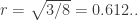 $r=\sqrt{3/8}=0.612..$ In fact, already for a unit triangle you need $1/\sqrt 3=0.577..$ In the wiki the number 0.563.. comes from projecting the facets of a non-unit edge length tetrahedron to the sphere such as the max diameter of the projected spherical caps is 1. Note that this is not attained between two vertices. At least you won’t run out of problems until your birthday…
  
  Reply
  1. ag24ag24 says:
    
    April 16, 2019 at 6:17 pm
    
    Damn! Thanks Domotor. Yeah, the triangles are “hyper-fattened”, I’d missed that. Ah well!
domotorp says:

April 16, 2019 at 5:46 pm

BTW, when thinking about colorings of spheres, I came up with another notion that is somewhere between tile-based and arbitrary colorings. Call a coloring (only) k-mixed if any point has a neighborhood where at most k colors appear. For example, it makes sense to study 2-mixed 3-colorings where color classes separated in a way. Unfortunately I cannot boast with any interesting discoveries, but I think it can be useful to classify colorings depending on how mixed they are.

Reply
1. domotorp says:
  
  April 16, 2019 at 5:48 pm
  
  “2-mixed 3-colorings where color classes separated in a way” should read “2-mixed 3-colorings, which means that color classes are separated in some sense”
  
  Reply
ag24ag24 says:

April 16, 2019 at 8:48 pm

OK here is another idea. On a sphere of any radius greater than 0.5, there is an x for which we can place four points A,B,C,D such that AB=BC=CD=AD=1 and AC=BD=x. If the radius exceeds about 0.543, x will be greater than about 0.6, which allows three points P,Q,R on that sphere to satisfy PQ=QR=x and PR=1. Let us suppose we can 3-colour such a sphere. Then we know that at least one of the pairs A,C and B,D must be monochromatic – but we also know that at most one of the pairs P,Q and Q,R can be monochromatic. Thus, I think this means that exactly half of the pairs of points at distance x must be monochromatic. Is that correct?

If so, it remains only to show that the “exactly half” option is impossible. I haven’t yet seen a way to do that – anyone?

Reply
1. domotorp says:
  
  April 17, 2019 at 10:26 am
  
  Nice! About a month ago I also had the ABCD part of this argument, but I haven’t realized that you can continue it with the PQR. Btw, why do you need x to be greater than 0.6? Isn’t 0.5 enough? Or you want to use it for some further arguments like in Prop 36?
  
  One issue (that we can think about later) is that the probabilities cannot be defined on the sphere as on the plane because of the Banach-Tarski paradox.
  
  Reply
  1. ag24ag24 says:
    
    April 17, 2019 at 11:06 am
    
    Thanks! I got 0.6 (actually 0.5996…) because we’re using chordal distances, so PR/x is less than 2 even when P,Q,R all lie on the equator (and as the radius falls, so do both x and PR/x). I’d forgotten about Prop 36 – does that complete the argument, or does the B-T paradox (which is waaay above my pay grade) mess it up?
    
    Actually I do now see that we can complete the argument for a countable infinity of radii (unless the B-T paradox intervenes?). Let PQ be x and P,Q bichromatic. Then we can identify two points R1,R2 at distance 1 from P and x from Q, which must both be the same colour as Q. But then there is also a point P2 at distance x from Q and 1 from R2, which is not the same colour as Q, so then there is a point R3 at xfrom Q and 1 from P2 that is the same colour as Q, and so on. For suitable radii, there will then be a finite number n such that Rn coincides with P. But of course there are also uncountably many radii for which there is no such n.
  2. domotorp says:
    
    April 17, 2019 at 3:39 pm
    
    Yes, I think that your argument is correct, except for the B-T paradox, because of which we cannot define $p_d$ . At least it shows that there cannot be a measurable coloring. Also, Prop 36 works, in fact, is even simpler. As you wrote, for any PQ of length x>0.6 there are two possibilities to find an R such that PR=1 and QR=x. Denote these by R1 and R2. If R1R2>0.6 (another condition about r), then we get that the triangle QR1R2 is monochromatic with probability exactly half and rainbow with probability exactly half. Creating a rhombus or parallelogram QR1R2S such that S is also at least 0.6 far from the other vertices, we get a contradiction as we have only 3 colors. I didn’t calculate how large a radius we need for this to work.
  3. ag24ag24 says:
    
    April 17, 2019 at 3:55 pm
    
    Ha, your post crossed with mine. Yeah, you had the same idea as me that R1,R2 must be different colours if they are different from Q. I don’t think your construction quite works as stated, because R1R2 could be too big to allow a triangle with third side 1, but my fix for that (iterating rotations) presumably works for yours too – and it also of course means that R1R2 can be arbitrarily small, so there is no new constraint on the radius after all. Ah, and I’m not seeing why your Q,R1,R2,S can’t all be the same colour – where is the contradiction?
    
    But anyway, regardless: how could we sidestep the B-T issue? It would be awfully nice not to have to assume measurability. Can you explain in simple terms why B-T implies that P_d is not defined?
  4. ag24ag24 says:
    
    April 17, 2019 at 5:26 pm
    
    OK, I have now understood why B-T implies that p_d is not defined – we basically get p_d = 2p_d.
    
    Suppose we had a set of points in which all 3-colourings make exactly half of the edges of length x mono (I don’t have such a graph but I bet they can be constructed from multiple copies of ABCD and PQR). Then presumably we could combine multiple copies of that using something like the construction I just derived, to create a bona fide 4-chromatic UD graph. I will think about that…
  5. domotorp says:
    
    April 17, 2019 at 5:42 pm
    
    Q,R1,R2,S can be monochromatic, but only with probability exactly half. I think this is exactly the same as in your crossposted argument (and also the same as Prop 36).
    
    Regarding B-T: The problem is that defining $p_d$ is not possible directly when the coloring is non-measurable. If you check the beginning of http://michaelnielsen.org/polymath1/index.php?title=Probabilistic_formulation_of_Hadwiger-Nelson_problem, you can see that it is done using some tricks and that the appropriate group is amenable. Unfortunately the same group is not amenable for the sphere (or any higher dimensional Euclidean space). I’m also not an expert of this topic, so I’m afraid I won’t be able to provide more details.
  6. domotorp says:
    
    April 17, 2019 at 5:52 pm
    
    Another crossposting… Anyhow, I would also think that the gadget can be usually combined to get a finite UD graph.
ag24ag24 says:

April 17, 2019 at 3:40 pm

OK, I think I have a way to eliminate the “exactly half” case (with the caveat that I still need Domotor to rule on whether the B-T paradox gets in the way). It’s a bit elaborate – maybe it can be streamlined.

Define x as a function of the radius as before (i.e. wrt my ABCD tetrahedron), and let the radius be strictly greater than the minimum value that allows a triangle of sides x,x,1 on the sphere. Since we are only interested in radii less than $1/\sqrt{3}$ , it turns out that x is always less than $2/\sqrt{6}$ = 0.8016…

Then let the distance PQ be x and the pair P,Q be bichromatic, and identify R and S as the points at distance x from Q and 1 from P. Define R2 as before – most simply, it’s the reflection of S in QR – and S2 as the reflection of R in QS. Then define Rn and Sn iteratively. Find the minimum n for which the distance RnSn (which hereafter we denote as y) is greater than x but small enough to let us make a triangle on the sphere with sides y,y,1. We won’t be using the intermediate Ri and Si below, so for simplicity we now just rename Rn and Sn to R and S respectively.

As noted earlier, R and S are the same colour as Q and thus each other. Now, for each P,Q-like pair there are two R,S-like pairs (i.e. pairs of points at distance y) – one at x from Q and 1 from P, and the other at x from P and 1 from Q. Conversely, for each R,S-like pair there are two P,Q-like pair there are two P,Q-like pairs (i.e. pairs of points at distance x) that give rise to that R,S pair. Also, because triangles of sides y,y,1 exist, we know that at most half of the pairs of points at distance y are mono. Since exactly half the pairs of points at distance x are mono, that means that NONE of the R,S pairs associated with mono P,Q pairs can be mono.

But now, we can rotate again. Consider a mono P,Q (say it’s colour 1) and let its R and S have colours 2 and 3 respectively. Then we identify T as the reflection of S in QR. Identify the point U that’s at distance x from Q and distance 1 from R and T. The U,Q pair must be mono, so T must have colour 3. So that means the pair S,T is mono (both colour 3). Now check whether the distance ST is in the range that allows triangles with two such sides and the third side 1. If it isn’t, keep going: make T2 as the reflection of S in QT, T3 as the reflection of T in QT2, etc until the distance STn does allow such a triangle, Rename Tn as T and let the distance ST be z. Note that T is an even number of steps from S (where the original R was one step from S), so we still have S,T mono.

But wait: that same pair S,T can also be constructed if we start with P,Q bichromatic, and in that case it’s also mono. So all pairs of points at distance z are mono – which is impossible because we can make a triangle with sides z,z,1.

Have I messed up?

Reply
1. domotorp says:
  
  April 17, 2019 at 6:00 pm
  
  I’m a bit tired and failed to fully digest this. My main concern is that if you can find far enough Rn and Sn, then why can’t we do the same in Prop 36 for every d? This would be a great improvement there.
  
  Reply
  1. ag24ag24 says:
    
    April 17, 2019 at 6:05 pm
    
    Well, just because in the plane we don’t have the equivalent of the ABCD tetrahedron that defines an x with p_x = exactly 1/2, so the argument can’t even begin. Right?
domotorp says:

April 18, 2019 at 4:40 pm

test

Reply
1. domotorp says:
  
  April 18, 2019 at 5:09 pm
  
  For some reason my comment won’t post, but you can read it here:
  
  Hello world!
  
  Reply
ag24ag24 says:

April 18, 2019 at 5:12 pm

I’m posting this for Domotor, who for some reason couldn’tget it to appear.

I might overlook something, but I think that something similar to your method will prove that in the PLANE we have $p_d \lneq 0.5$ for every $d \gneq 0.5$ .
Proof. Take a circle of radius d centered at O. Pick a point A1 on the circle. Let B1 be another point on the circle such that A1B1=1. Let A2 be another point on the circle such that B1A2=1, etc. Assume $p_d=0.5$ . Then (with probability 1) either each Ai has the same color as O, or each Bi has the same color as O. Pick 4 indices i1,i2,i3,i4 such that 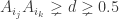$A_{i_j}A_{i_k} \gneq d \gneq 0.5$ for any pair j,k. This can be indeed done except for a few $d\gneq 0.5$ , for example $1/\sqrt 2$ (but luckily we already know that the statement holds for these d from earlier proofs). But then for any distance $x=A_{i_j}A_{i_k}$ we know that $p_x\le 0.5$ , and from our assumptions, also $p_x=0.5$ due to our construction. Moreover, since all the Ai are monochromatic at the same time, also all of them need to be different from each other (and from O) at the same time. But this is impossible, as we have only 4 colors.
Note that the upper bound we get from this proof tends to 0.5 as d tends to 0.5.

What I like in this proof (if it’s correct) is that the only fact it uses about the number of colors that it’s less than the kissing number. So let me conjecture (why not?) if nobody has done so before that the chromatic number of any $\mathbb R^n$ is equal to its kissing number.
Come to think of it, we don’t even need this if we slightly alter the construction; instead of rotating always around O, we could also rotate around any Ai (as is also done in the proof of Prop 36), so the bound $p_d \lneq 0.5$ holds for every $d \gneq 0.5$ for any number of colors. (This kind of makes my conjecture ill-funded but it’s so nice that I’ll go with it anyway.)

Reply
1. Bernhard Hockertz says:
  
  April 18, 2019 at 7:21 pm
  
  Though I don’t think I’ve heard the kissing number/chromatic number conjecture anywhere else before explicitly, I think I’ve seen it at least implied. I’ve also briefly conjectured in this direction myself when I first heard about the E_8 and Leech lattices. My thoughts went to Permutohedron constructions since those have a lot of great properties for tesselating spaces, and assuming that the most efficient coloring is based on Permutohedrons, or something similar I’d be fairly certain the the chromatic and kissing number are at the very least very closely related. Something like… CN=KN+n-1 or what have you. There’d have to be some sort of very similar structure.
  
  What threw a wrench into those thoughts were the arc boundary tesselations I first saw thanks to Aubrey. It was also around this time I lessened my focus on the geometry and instead started stabbing at the fundamental constraints with topology, set and measure theory, of which the last is the only really tough customer, on which I just can’t seem to find the necessary intermediate steps no matter what I do.
  If I had to conjecture then we don’t have the flexibility to actually find a 6-color tesselation of the plane, and non-tile based colorings are off the table anyway.
  With 3 dimensions I can certainly imagine a super specific arc boundary severing enough connections to push the chromatic number down to 14. Maybe even 13, though I doubt that.
  12 though as with the kissing number? Having spend weeks on the according Honeycomb I can’t even begin to fathom what sort of shape would severe enough connections to drop 3 whole colors.
  
  I’m curious to look into the possible connections between KN and CN but I’m blanking on any concrete conjecture to chase. For now I’m busy with the video a few more days anyway. Since the deadline has passed… I’ll just put some extra details in, try and make this accessible and understandable to a wide audience. It was certainly nice to see the patchiness in Heule’s 553 graph animated and highlighted.
  
  Talking about the passed deadline… now what? Is this place gonna actually be locked some time or will there just be no new threads/wiki updates?
  
  Reply
  1. domotorp says:
    
    April 19, 2019 at 1:15 am
    
    Yeah, CN=KN+n-1 seems more plausible.
  2. Bernhard Hockertz says:
    
    April 19, 2019 at 2:25 pm
    
    Something about this kept popping into my mind regularly since yesterday.
    
    So, on one side we have highly regular structures, such as permutohedra honeycombs and lattices.
    On the other side we have arc boundary constructions and a looming possibility of non-lattice arrangements for kissing numbers too.
    
    A deeper look at different types of tesselations, their duals and also other ways of turning one honeycomb into another has generally shown to me that in 2 and 3 dimensions there doesn’t seem to be too much hope for better chromatic numbers than 7 and 15 respectively. Arc boundaries can sever some connections, but we need a lot of severed connections to drop even a single color.
    
    If however there are non-lattice kissing numbers, I would assume most likely in the dimensions leading up to those with new extreme symmetry (such as 8 and 24) I could see how they at the same time might predict less symmetric most efficient tesselations, using arc boundaries to drop needed colors below what a more universally symmetric construction can do. If so then the CN and KN might respectively be bound not to one most efficient rule of tesselating, but 2 (or more) that alternate depending on the number of dimensions and resulting possible symmetries.
    
    I suppose this might be a conjecture I could chase… many years down the road if I keep my hobby investment and fascination with this up for so long.
    Though the idea sounds interesting to me, I think actually looking into it further is way above my head for now. I’ll just keep it around here to look back on in case I decide to go for it some other time.
ag24ag24 says:

April 18, 2019 at 6:06 pm

I think I follow that… yeah I think it works! Basically you are extending my approach simultaneously to the (up to) six distances between your four A’s – right?

By the way, I just dug out what someone told me way back in the first thread about strict inequality symbols: within the latex dollars you can still use “& l t ;” and “& g t ;” to get the simple angle brackets. (Without the spaces, of course!)

Nice conjecture! It seems to be consistent with what’s known… the numbers at https://en.wikipedia.org/wiki/Kissing_number_problem stay between the known asymptotic bounds on CN for R^n. I haven’t found whether there are known asymptotic bounds for the kissing number.

Reply
1. domotorp says:
  
  April 19, 2019 at 1:19 am
  
  Yes, I also couldn’t find anything about it, except for these complicated bounds in the comments section here: https://oeis.org/A257479
  
  Reply
Jaan Parts says:

April 20, 2019 at 2:48 pm

Some thoughts towards the human-verifiable proof (for the chromatic number of the plane $\chi\ge 5$ ).

Starting from graph $\oplus^4 V_{31} = V_{31} \oplus V_{31} \oplus V_{31} \oplus V_{31}$ I have found 409-vertex graph with Euclidean radius only $4/3$ and monochromatic pair of vertices with coordinates $(–4/3, 0)$ and $(4/3, 0)$ in 4-coloring (see picture below).

Vertex coordinates are available here:
https://www.dropbox.com/s/msbtrhd5gs8ajsn/g409c.vtx?dl=0

This graph has 409 vertices, 2046 unit-distance edges, 912 cliques, 186 Moser’s spindles, vertex degree in range 6…30. It includes 17 unit-distance 7-vertex wheels, 12 unit-distance 6-vertex almost-wheels (see yellow, green and blue vertices) and three 8-vertex constructions (including monochromatic pairs of vertices), which I called the sliding bridge (see blue vertices). Interestingly, a similar bridge appears also in more compact graphs with other Euclidean distances between equally colored vertices in 4-coloring.
The graph allows further reduction (397-vertex with 4-fold symmetry). Two copies of such graph with an additional edge lead to 5-chromatic graph. This is not so far from record graphs of Marijn Heule. In some ways, the resulting 5-chromatic graph is even simpler, since it splits into two subgraphs, connecting only at two vertices, and has a fairly strong 12-fold symmetry.

The graph has the following additional properties in 4-coloring:
– all 5 wheels centered at the graph origin (shown in yellow) cannot contain a monochromatic triple;
– all 6 wheels with centers on a radius of $\frac{\sqrt{11} – \sqrt{3}}{6}$ from graph origin (some of green vertices) cannot contain a monochromatic triple;
– all large diagonals of 6 rhombuses that make up the bridge (see blue vertices) cannot be monochromatic (that is, this gives virtual edges with lengths of $5/3$ and $\sqrt {11/3}$ )
It remains to figure out what caused these properties and how they force a pair of extreme vertices of the bridge have the same color.

Reply
1. Jaan Parts says:
  
  April 20, 2019 at 2:54 pm
  
  I try to write not parsed expressions differently (it seems used minus sign causes error):
  $(-4/3, 0)$
  $\frac{\sqrt{11} - \sqrt{3}}{6}$
  
  Reply
2. domotorp says:
  
  April 20, 2019 at 4:51 pm
  
  What I would be very interested to know is how much smaller these graphs can be if we combine them with the results of the probabilistic approach. We can use 0 < $p_d$ > 0.5 for a wide range of values; for simplicity, suppose we could use it for all d. This would mean that we can add two additional edges to a unit distance graph or, alternatively, we can merge any two vertices of a unit distance graph to obtain a new graph whose chromatic number is still a lower bound for the CNP. Would any of these tricks significantly reduce the number of vertices in your constructions?
  
  Reply
  1. domotorp says:
    
    April 20, 2019 at 4:52 pm
    
    Of course I’ve meant to write 0 < pd < 0.5, just these codes are driving me nuts…
  2. Jaan Parts says:
    
    April 20, 2019 at 5:15 pm
    
    Hmm, I did not understand the question. I have to get into the probabilistic formulation first.
  3. domotorp says:
    
    April 20, 2019 at 5:28 pm
    
    You needn’t get into it at all. My first question is what if two of your edges needn’t be unit edges, how much would that decrease the number of vertices? My second question is what if two given vertices need to have the same color, how much would that decrease the number of vertices?
  4. domotorp says:
    
    April 20, 2019 at 5:31 pm
    
    As an example, note that if we ask the same question with three non-unit edges instead of two, then the answer is that 5 vertices suffice, as K5 can be realized (with 7 unit edges and 3 non-unit edges).
  5. Jaan Parts says:
    
    April 21, 2019 at 3:13 pm
    
    I did not do such research and do not quite understand what the point is. Could you clarify the purpose?
  6. domotorp says:
    
    April 21, 2019 at 4:22 pm
    
    The point is that if this operation makes the graph small enough so that it becomes human verifiable that the chromatic number is 5, then we have a proof for CNP least 5 that doesn’t use a program.
  7. Jaan Parts says:
    
    April 21, 2019 at 4:39 pm
    
    Yes, but we only have edges of unit length to do that. I still do not understand.
  8. ag24ag24 says:
    
    April 21, 2019 at 5:30 pm
    
    Let me try. Suppose we had proved that $p_{\sqrt{3}}$ and $p_2$ are both less than 1/3. Then, we would immediately know that the CNP is at least 5, because there exists a 5-vertex graph (namely, half a hexagon) that has only three non-unit inter-vertex distances, all of which are either $sqrt{3}$ or 2, and which thus must have one of those three vertex pairs mono in any 4-colouring, whereas with those upper bounds on the probabilities there must, in any colouring of the plane, be some half-hexagon somewhere in the plane that has none of those three vertex pairs mono, and that therefore has all five vertices being different colours.
    
    So now, in reality we do not have any such bound (though I wonder if we might get it for $p_{1/\sqrt{3}}$ ). What we do have, though, is that p_d is less than 1/2 for all d greater than 1/2. Therefore, the equivalent logic works if we have a graph in which there are two specific vertex pairs, A,B and C,D, such that in any 4-colouring of the graph either A and B are the same colour or C and D are the same colour. Obviously we already have such graphs, since in your graphs we can dispense with C,D. But with that relaxed condition, it should be possible to remove vertices. The question is, how many? It is tantalising that the geometric mean of 5 and 409 is only 45… if we could find such a graph with under 100 vertices, it’s a fair bet that we could prove the property without a computer.
    
    The next question is where to begin. I think the most promising line of attack would be to use two of the 8/3 pairs in your 409er, so let’s say $[(2/3,2/\sqrt{3}),(-2/3,-2/\sqrt{3})]$ and $[(2/3,-2/\sqrt{3}),(-2/3,-2/\sqrt{3})]$ . They start out both needing to be mono, and the relaxed property is that one or other of them is mono.
    
    If this works it will be so cool. It was one of he main original goals of the project, and it’s already the result of substantial input from several of us.
  9. ag24ag24 says:
    
    April 21, 2019 at 5:32 pm
    
    Jeez I made a mess of that. I think everything is reasonably intelligible, but Dustin please fix things if you have a moment.
    
    [Done! – M.]
  10. Jaan Parts says:
    
    April 22, 2019 at 12:26 pm
    
    Thank you, Aubrey. Something starts to clear up. But again there are more questions than answers.
    
    All three pairs of vertices with distances of 8/3 in the 409-vertex graph are monochromatic. Why do we need to weaken this statement and say that at least one of them is mono? What does this give?
    
    Does the probabilistic argument take into account that if we take several non-unit distances, then, generally speaking, the probability of one event depends on the probability of another? What if, for example, in the presence of one monochromatic pair, the probability of the formation of another sharply increases? (Or is it impossible or does not change the overall logic?)
    
    It is not clear how the geometric mean appears.
    
    Is it normal that some lower bounds (on a wiki page, for example, for 8/3) are greater than upper bounds?
  11. ag24ag24 says:
    
    April 22, 2019 at 1:11 pm
    
    I’ll answer those questions in increasing order of difficulty!
    
    3) My comment about the geometric mean was really jsut frivolous speculation. I have no real reason to suppose that the smallest graph with one of two specified edges mono will have somewhere near that number of vertices. Please ignore that.
    
    4) The cases where the lower bound is greater than the upper bound are simply those that lead directly to the proof that the CNP is greater than 4. Remember that the table is for 4-colourings: I think the only things we know about higher-order colourings are that p_1 is 0 and p_d is less than 1/2 for all d greater than 1/2.
    
    1) The only reason for weakening the statement is that then it is likely that the graph can be smaller – maybe much smaller. One of the main goals of Polymath16 is to find a proof that the CNP is at least 5 that does not rely on computers to verify any properties of any graph. Domotor’s cool realisation is that we would obtain such a proof if we could find a reasonably small graph that has at least one of two specified vertex pairs (both of which must be more than 1/2 apart, of course) the same colour in any 4-colouring. The smaller the graph, the shorter the proof that it has that property; therefore, the hope is that we can find a small enough graph that the proof is human-derivable (in a publishable number of pages!).
    
    2) The probabilities are actually not dependent on each other, because they are not defined in terms of any particular location or orientation of any particular graph in the plane – they are defined in terms of all such locations and graphs. The statement “p_d is less than 1/2” simply means that in any 4-colouring of the plane, fewer than half of the pairs of points at distance d from each other are the same colour – no graphs mentioned yet. So then if p_d1 and p_d2 are both less than 1/2 and we have a graph that has vertices A and B that are d1 apart and also two vertices C and D that are d2 apart, and then we colour the plane, then we know that out of all the infinitely many places and orientations that we can place our graph in the plane, there will be some in which A and B are different colours and C and D are also different colours, because fewer than half of those infinitely many copies of our graph have A and B the same colour and also fewer than half have C and D the same colour. (I’m playing fast and loose with fractions of infinities, of course, but that’s OK in this case, trust me.) So if we have a graph in which either A is the same colour as B or C is the same colour as D in any 4-colouring, we have a contradiction, which means CNP must be greater than 4 (because the P_d’s are all defined in terms of 4-colourings of the plane). Note that d1 and d2 can be equal; in the case I’m suggesting you explore, they are both 8/3.
  12. Jaan Parts says:
    
    April 22, 2019 at 2:20 pm
    
    It seems to have come to me. It is proposed to throw out vertices from the graph until at least one of the two fixed pairs remains monochromatic. (And when it will be clear with the proposed four of vertices, play with all possible combinations of fours up to isomorphisms.) So?
  13. ag24ag24 says:
    
    April 22, 2019 at 2:37 pm
    
    Yes, exactly, throw out as many vertices as you can without allowing a 4-colouring in which neither of the two pairs is mono. I don’t think there is any need to look at other pairs of vertex pairs, because you would be starting from a weaker condition on the 409er and thus it is very unlikely that you can delete a larger number of vertices than with the suggested pairs while still retaining the required property. (We really need a name for the property: I’m going to call it “semi-mono”.) When you have your minimal semi-mono graph, show it to us and we’ll all see whether we can figure out a human-comprehensible proof that it is semi-mono.
3. ag24ag24 says:
  
  April 22, 2019 at 2:21 pm
  
  Addendum to answer 2: of course the generalised version of Lemma 17 also applies for any number of colours.
  
  Reply
ag24ag24 says:

April 21, 2019 at 1:52 pm

Many thanks Jaan – a lovely graph! Not sure there is all that much in it that is fundamentally new, though – we already had graphs enforcing mono at distance 8/3 (Jannis and Marijn; see the second thread, posts starting on April 28th), and the rhombus properties follow directly from that – but it’s great to have a compact one with so many triangles that can’t be mono.

I feel we really ought to look hard at building graphs with a lot of edges of length 8/3 and spindlings thereof. If we can find one that (for example) forces just one 6-wheel (of a component Parts graph, presumbly) to have a mono diagonal in any 5-colouring, the chase would be on for a counterpart of my graph L that requires a mono triangle in any 5-colouring. Or of course there could be much more elaborate clampings, such as in Geoff and Dan’s “new proof” paper.

Reply
1. Jaan Parts says:
  
  April 21, 2019 at 3:19 pm
  
  Yes, you are right about rhombuses. But I meant reverse causation.
  
  Reply
2. Jaan Parts says:
  
  April 21, 2019 at 3:34 pm
  
  I set myself the task to get an analogue of a half-Moser’s diamond for 4-coloring. Graphs of Marijn are not suitable because they require multiple links between subgraphs. The graph of Jannis is not compact.
  
  Reply
Jaan Parts says:

April 21, 2019 at 3:00 pm

Trimming the graph $\oplus^4 V_{43}$ , I obtained a graph with Euclidean radius of $1.02$ and distance $8 / \sqrt {27}$ between two vertices with the same color in 4-coloring. Minimum radius of such graph is somewhere between $1$ and $1.02$ .

Reply
1. ag24ag24 says:
  
  April 21, 2019 at 3:05 pm
  
  Nice! Show us! The spindling of two of those must be really close to fitting inside a 4-tileable shape.
  
  Reply
2. Jaan Parts says:
  
  April 21, 2019 at 3:22 pm
  
  The picture is not interesting: too many vertices (several thousand).
  
  Reply
  1. ag24ag24 says:
    
    April 21, 2019 at 3:42 pm
    
    Oh, it’s still interesting because of the 4-tileable question (above). What are the coordinates of the two forced-same vertices? Also, is the graph still hexagonally symmetrical? If so, I bet you can find lots of specific radii less than one at which you can remove the vertices without losing the forced-same property.
  2. Jaan Parts says:
    
    April 21, 2019 at 3:58 pm
    
    It is 12-fold symmetric (hexagonal). Forced vertices coordinates are $(0, \pm 4/ \sqrt {27})$ .
    I did everything I could to thin the graph while maintaining symmetry. I do not think that it is possible to significantly reduce the number of vertices due to the loss of symmetry.
3. Jaan Parts says:
  
  April 21, 2019 at 3:46 pm
  
  Judge for yourself. Numbers are vertex degrees. This is a reduced version already.
  
  Reply
domotorp says:

May 2, 2019 at 8:19 am

Let me ask another question before the project goes silent for another half year. Is there a finite coloring of the plane avoiding unit distances that has an arbitrarily small period? So for example, I would like that col(p)=col(q) for every p and q if the differences of their respective coordinates are both of the form 2/(2k+1) for some k.

Reply
1. ag24ag24 says:
  
  May 2, 2019 at 2:12 pm
  
  I’m not understanding why this isn’t trivially true. Since one is not constraining the number of colours, surely for any period x that is not the square root of the reciprocal of the sum of two squares one can just use a tiling using sufficiently small squares (i.e. of side x/n for some sufficiently large integer n, and using n^2 colours), since there is then no pair of squares whose centres are exactly 1 apart?
  
  Reply
  1. domotorp says:
    
    May 2, 2019 at 4:42 pm
    
    I mean that I want a coloring with a finite number of colors for which every 2/(2k+1) is a period.
  2. ag24ag24 says:
    
    May 2, 2019 at 9:03 pm
    
    Now I’m very confused. Originally you said “for some k”. One interpretation of your sentence is that different point-pairs p,q can use different k, but I presume you intended that no, it’s always the same k for every point-pair. My construction does that – specifically, my x is your 2/(2k+1).
    
    But now you say “every 2/(2k+1) is a period”. I don’t see how a colouring can be periodic at infinitely many different distances, so I must be totally misunderstanding.. Sorry if I’m being dumb!
  3. domotorp says:
    
    May 3, 2019 at 1:27 am
    
    It can be if it is not tile-based, for example, color the rationals blue and the irrationals red. Such colorings can be also derived from p-adic valuations as I’ve learned recently, see this paper: https://msp.org/pjm/1982/99-1/pjm-v99-n1-p03-s.pdf
  4. Bernhard Hockertz says:
    
    May 3, 2019 at 4:29 am
    
    I’m also not sure I understood it completely. Are you talking a about a coloring of the whole plane with finite colors, or a coloring of a finite subgraph of the plane?
    
    A non-tile based coloring of the whole plane (UD, Euclidean) or higher dimensional spaces requires aleph_1 colors if my topological approach is even just roughly correct. Only on a numberline does the non-tile based approach yield full colorings with finite colorings, and chromatic colorings too at that.
  5. domotorp says:
    
    May 3, 2019 at 5:18 am
    
    I’m talking about a coloring of the whole plane with finite colors. I’m very happy to see if you can disprove the existence of a coloring with an arbitrarily small period that avoids the unit distance.
  6. Bernhard Hockertz says:
    
    May 3, 2019 at 7:16 am
    
    I’ve always had less than full confidence in my old topological approach, and a moment ago I finally figured out the leap in logic I made that has eluded me for over a year. That nagging piece of “this seems too easy to be the whole story”.
    To be clear, I still think that my statements on that front are correct, but for somewhat different reasons. I’ll get into those in a moment, but first let me make clear that this still only holds for non-tile based colorings. I’m not deep into periodicity&co, so any statements on the tile based side will have to be made by someone else.
    
    Alright, so first let’s look at how non-tile based colorings work in 1-dimension. What we are really strictly speaking about when saying non-tile based colorings here is a coloring using 0-manifolds, points, in such a manner that for every point with color x, in every direction there is another point with a color that is not x, and which is arbitrarily close at that.
    Specifically in 1-dimension we could color the interval [0,1) with rational numbers having color x, and irrational numbers color y. So long as we then color the rest of the numberline accordingly we never have a continuous single-colored interval, yet still use only 2 colors. Note that on the numberline we also only have 2 directions to cover.
    
    In 2 or more dimensions we have $\aleph_1$ directions to cover though. Let’s try to think about a small area, only 2 colors. We could use the rational/irrational coloring scheme and rotate it, but by doing so we’d create rings, which are single-colored 1-manifolds, so we already lost. In general this dynamic, though I don’t quite know how to describe or analyze it really properly yet, is where the issue lies, I would think. If we have a point with color x then in $\aleph_1$ directions we need another color arbitrarily close, and all of those $\aleph_1$ points need a different color arbitrarily close in $\aleph_1$ directions.
    
    Now the hard proof is missing here, but this conclusion is also the only thing that squares properly with the other hard proves. I certainly have something new to think about now. There might also be a way to square it with my other much more solid and specific proof I’m not seeing yet.
  7. Bernhard Hockertz says:
    
    May 4, 2019 at 6:46 pm
    
    I might be eating my previous words with this, but maybe a given area can be colored without tiles with finite colors using a shelled rational/irrational approach? If that works then a given n-volume in $\mathbb{R}^n$ would require n+1 colors. So 2 for a numberline, 3 for the plane. This would still force us to use a lot more colors than necessary for a chromatic coloring using tiles, but “tiling” with this non-tile n-volume would then lead to a finite amount of colors. CNP*3 in this case. I’m not really sure either way though anymore.
    
    I doubt this is overly helpful.
    Though I guess I found an error with my earlier stuff and some interesting things to think about.
  8. Bernhard Hockertz says:
    
    May 8, 2019 at 3:37 am
    
    Since you said “It can be if it is not tile-based”, is there a proven issue if it’s tile-based?
    What if the coloring isn’t tile based, but trivially convertible to one that’s tile-based?
    
    That is could a non-tile based coloring that’s trivially convertible still do what you’re asking for?
  9. domotorp says:
    
    May 8, 2019 at 11:23 am
    
    If it is tile-based with arbitrarily small periods in both the x- and y-direction, then it has to be constant.
Jaan Parts says:

June 19, 2019 at 4:33 pm

I have some results (if you think the lack of a results is the result). Just in case, I decided to publish, suddenly come in handy.

1. I think that in the task of searching for a 6-chromatic graph it would be nice to have a certain indicator of density of the fifth color. It is assumed that it should increase to a certain critical value, when five colors would be insufficient. For the role of such an indicator to begin with, one can suggest the minimum number of vertices that should be removed to reduce the chromatic number of the graph by one (from 5 to 4). For example, in the family of Marijn’s record graphs, it suffices to remove one single vertex, so the fifth color density is here minimal.
I tried to calculate this indicator with the help of MaxSAT (the open-wbo program was used). The result was not very encouraging. Already for a graph with slightly more than 1000 vertices and three vertices that require the fifth color, the calculations last more than two days (I had to interrupt the execution of the program). The question arises: what alternatives can be offered here?

Reply
1. Bernhard Hockertz says:
  
  June 20, 2019 at 3:25 am
  
  I’d be curious too. I’ve been thinking about this density as well as coloring efficiencies on and off, but… suffice to say I have nothing really to show aside from a small bit of intuition.
  
  There might be some mileage in the n-ball graph approach though. So far I’m certain of how they can explain why coloring in 2 or more dimension requires tiles, and it should set the stage for understanding how close vertices are “pressured” into having the same color. What we’re seeing is that the more vertices there are, and the fewer colors we use, the more close vertices will be forced into the same color. In the infinite case this is what leads to the necessity of tiles, and even in the finite case, with sufficiently dense graphs and few colors, it leads to certain necessary patterns. I’d wager this should be adaptable into computational optimizations… somehow. If so, then a lot of patterns can simply be ignored up front. If I were to guess more specifically I’d say that there should be some minimum diameter of single-colored n-balls that should be present to allow for an efficient coloring of both infinite and finite graphs, and all cases without those can be ignored. This optimization could then be applied to all colors, except the last, of which we want as few vertices as possible. If that can be proven it should help a lot, right?
  Thinking about this I just took a look at the Golomb graph again, and when we constrain the 4th color to the center node, of course 3 colors in the triangle, and then again the 3 colors in a repeating pattern in the hexagon, then we can rotate the color in the hexagon so that same colors in the hexagon are either closest, or at medium distance to the counterparts in the triangle, but if we disperse the colors with maximum distance it doesn’t work anymore.
  The problem being this is just conjecture by me, and I’ve been focusing primarily on the infinite case. I’m not sure what the exact rules would be, how to prove them as of yet, and even then, how to program and use them.
  I’m also still working on the n-ball graph video, just taking time with it and polishing it since the deadline is long passed anyway, but I’ll keep this conjecture in mind and will try looking into it eventually, possibly make a video on that too… in many months that is.
  
  Reply
2. Jaan Parts says:
  
  June 20, 2019 at 4:44 pm
  
  I don’t have the sure impression that the concentration of colors (localization of mostly one color in a certain area of the graph) is the rule. Now I can only remember Marijn’s conclusion that there is a confirmed tendency for vertices of his graphs that are close to distance 2 from the origin to have the same color as the origin.
  I also observed the effects of colors concentration for some graphs, but for other similar graphs I observed very motley colorings without any color patterns. The appearance of such patterns can be caused not by some kind of “pressure”, but by completely different reasons, for example, by vertices sorting method before running the coloring program.
  Do we really have already sufficient grounds to assert that on average such a concentration of colors takes place?
  The example with Golomb graph is also not clear for me. Let the center have color 4, the inner triangle – colors 123, the outer perimeter – 121213. Where is the color localization here?
  
  Reply
  1. Bernhard Hockertz says:
    
    June 20, 2019 at 6:47 pm
    
    For the Golomb graph the case I looked at used colors 4, 132 and 123123 respectively. There’s only 3 possible rotations of the outer (or alternatively the inner ring) possible of which only 2 work. The one that doesn’t has a collision with all of the first 3 colors, and is the one with the biggest distance between the vertices of the first three colors. where no vertex of color 2 for example is closer to another vertex than unit distance, whereas the 2 working examples have less than unit distances. That being said, it’s more a curious case than anything that can really prove stuff.
    
    This patchiness was discussed all the way back in the fifth thread. Notable quote by Heule himself about the graph in question:
    “Although I did not force the patchiness, I did force all vertices apart from the origin to be colored with 4 colors. Without that restriction the patchiness would disappear.”
    
    And to be clear, there is no patchiness whatsoever to be expected if the restrictions on graphs aren’t strong enough. However as in your case, using the minimum number of colors and restricting the last color to as few vertices as possible should definitely force patchiness even in finite graphs.
    I’ll go into more detail in my video. The origin of this patchiness and some necessity can be proven using n-ball graphs. The short gist is that 2 vertices at unit distance embedded in a space and expanded by some radius yield 2 n-balls that can absolutely strictly only be colored solidly, one and only one color per n-ball. This is equivalent to how a bipartite graph can’t be colored when any vertex contains 2 or more colors instead of just one. But in this case the n-balls act like finite vertex counterparts themselves.
    And this property holds generally, any finite graph can be embedded and expanded this way, yielding a functionally equivalent n-ball graph where some (not necessarily all) n-balls can only contain a single color.
    
    To put it in yet another way, if we could efficiently color 2 or higher dimensional spaces with unit distance edges without using tiles, or more specifically at least some solidly colored areas, then by extension we would be able to come up with chromatic colorings for finite unit distance graphs where all vertices have multiple colors, which is clearly a contradiction.
Jaan Parts says:

June 19, 2019 at 4:34 pm

2. I decided to continue the search for graphs with large values of the fractional chromatic number (FCN), and bring it to at least 3.98. There are all prerequisites for this. The main problem here is not to find the actual graph, but to calculate the FCN value, since this is a long process. A new graph, as a rule, is obtained by adding a certain set of vertices to the previous record graph (and, possibly, by removing some number of “weak” vertices). To speed up the process, it is convenient to operate with orbits instead of individual vertices, that is, sets of vertices (while sacrificing a little the optimality of the resulting graph in terms of used vertices). In the case of large graphs, the task is to search for such orbits that give not only the maximum increment of the FCN value when added to the initial graph, but also the minimum increase in the computation time (which can be estimated in the first approximation by the time of one iteration of the computational algorithm and even by part of this iteration).
Currently, FCN values are calculated for several subgraphs of a 799-vertex graph with (the record FCN is 3.971119), while the iteration duration (about 50 hours) almost does not change when the number of vertices varies from 547 to 799. I spent a lot of time on the family of subgraphs of 1201-vertex graph. It seems that its FCN is more than 3.99, but the iteration duration exceeds all reasonable limits (approximately 30 times more than for a 799-vertex graph), so it makes sense to look for a suitable subgraph with not very long computation time. With the mentioned 1201-vertex graph I observed (not for the first time) an interesting effect of the latching of the algorithm on the value FCN = 4. This problem was overcome, but as it turned out, an error appeared in the calculations, and this threw me back a month.

Reply
Jaan Parts says:

June 19, 2019 at 4:39 pm

3. Several (not very) new species to the zoo of 5-chromatic graphs.
About a month ago I was interested in the graphs of Tamas and Jannis, which in a certain sense give a very compact description, since used subgraphs involve a reduced number of rotations. For example, the graph of Tamas (https://dustingmixon.wordpress.com/2018/04/22/polymath16-second-thread-what-does-it-take-to-be-5-chromatic/#comment-3970) uses only three rotations at angles that are multiples of $\arcsin (1/ \sqrt{12})$ instead of the usual five (in Aubrey’s and Marijn’s graphs). I did not succeed in getting closer to answering the question why this is enough. It turned out only to slightly reduce the order of the graph (from 6937 to 5053) and to establish that from 8 subgraphs with different combinations of angles $\arccos (7/8)$ you need at least 5 to keep the chromatic number $\chi=5$ .
While playing with graphs, I found that the construction $(V \oplus V \oplus H) \cup \omega_4 (V \oplus V \oplus H)$ is redundant. The truncated graph $(V \oplus V \oplus H) \cup \omega_4 (V \oplus V)$ also has the chromatic number $\chi=5$ .
Here we use the usual notation for the 7- and 31-vertex graphs $H=W_7$ and $V=\bigcup_{n=-2}^2 \omega_3^{n/2} H$ and rotation multipliers $\omega_t = \exp( i \arccos( 1 - \tfrac{1}{2t} ))$ . Further it will be more convenient to use notation, in which the list of integer coefficients is explicitly given for the rotation multiplier $\eta=\omega_3^{1/2}$ . It is proposed to give this list as a superscript after the designation of the base graph. For example, $V=H^{\left\{-2,-1,0,1,2\right\}}=H^{\left\{-2...2\right\}}$ , and the entry $i\sqrt3H^{\left\{1\right\}}$ means the rotation of the graph $H$ by the angle $\pi/2 +\arcsin (1/\sqrt{12})$ and scaling $\sqrt3$ times.
In the proposed notation, the Jannis’s graphs $V_a \oplus V_x \oplus H \cup V_b \oplus V_y \oplus H$ and $V_a \oplus V_z \oplus H \cup V_b \oplus V_y \oplus H$ (https://dustingmixon.wordpress.com/2018/04/14/polymath16-first-thread-simplifying-de-greys-graph/#comment-3950) have the following subgraphs: $V_a=H^{\left\{-2,-1,1,2\right\}}$ , $V_x= H^{\left\{-2,-1\right\}}$ , $V_z= H^{\left\{-1,1\right\}}$ , $V_b=\omega_4 H^{\left\{-2,-1,0,1,2\right\}}$ , $V_y=\omega_4 H^{\left\{0,1\right\}}$ . Note that the list of vertices for the graph $V_z$ was given with an error.
Let us return to the graph $(V \oplus V \oplus H)\cup\omega_4(V \oplus V)$ . It has the form $G=L \oplus \omega_4 S$ , that is, it is divided into two subgraphs, large one $L$ and small one $S$ in Marijn’s terminology. It is not possible to construct a large subgraph using 2-fold Minkowski sum while keeping $\chi=5$ . But one can try to do this by adding a certain number of vertices to the base graphs. So I came to the base graph $V_{49}=H^{\left\{-2...2\right\}}\cup\frac{i}{\sqrt3} H^{\left\{-1,0,1\right\}}$ . Here is a drawing of this graph:

The result is a construction that uses only 2-fold Minkowski sums, which may be of some interest: $L= V_{49}\oplus V_{49}$ , $S=V\oplus V$ . In particular, it gives not only a more compact graph than $V \oplus V \oplus H$ , but also leads (unlike the latter) to a rather compact large subgraph by further reducing. Thus, it is possible to obtain a reduced large subgraphs $L_{451}$ (451 vertices, 29 orbits, symmetry order 24) or $L_{418}$ (418 vertices, 73 orbits, symmetry order 6).
Further work in this direction allows us to obtain even more compact subgraphs. For example, $L_{727}=V_{49}\oplus V_{37}$ (727 vertices, 4116 edges), $S_{361}=V_{31}\oplus V_{25}$ (361 vertices, 1746 edges), where $V_{49}=H^{\left\{-2...2\right\}}\cup\frac{i}{\sqrt3} H^{\left\{-1,0,1\right\}}$ , $V_{37}= H^{\left\{-1,0,1\right\}}\cup\frac{i}{\sqrt3} H^{\left\{-1,0,1\right\}}$ , $V_{31}= H^{\left\{-1,0,1\right\}}\cup{i}{\sqrt3} H^{\left\{-1,1\right\}}$ , $V_{25}= H^{\left\{-1,0,1\right\}}\cup\frac{i}{\sqrt3} H^{\left\{0\right\}}$ . In this version, the small subgraph is also well reduced to $S_{181}$ (181 vertices, 13 orbits, symmetry order 24) or $S_{151}$ (151 vertices, 26 or 29 orbits, symmetry order 6). This gives a total reduced 5-chromatic 568-vertex graph, which is not too far from Marijn’s record graphs. Here is a list of vertices of this graph (568 vertices, 2922 edges):
https://www.dropbox.com/s/21sly4f9lr41myl/g568.vtx?dl=0

Reply
1. domotorp says:
  
  June 20, 2019 at 3:54 pm
  
  I think that these are very interesting and might reduce the vertex count to a new record. I wonder what happened if instead of taking the union of two graphs (L and S), we take the union of three or four (all being 2-fold Minkowski sums).
  
  Reply
2. Jaan Parts says:
  
  June 20, 2019 at 5:36 pm
  
  It’s too early to talk about a record. On this way it is problematic to step below the 500 vertices threshold. I think that this is either impossible, or it will require fundamentally different approach. Perhaps it will be an increase in the number of subgraphs (although at first glance this should only worsen the matter). Do you have in mind here any particular construction like a few rotations with angles that are multiples of $\arccos(7/8)$ ?
  What is really interesting from my point of view is the fact that it is possible to get almost the same results from a rather compact graph with a simple reduction as from a large initial graph with significant amount of computation. Moreover, many vertices of the final graphs coincide. There must be something here.
  
  Reply
  1. domotorp says:
    
    June 21, 2019 at 1:02 am
    
    Unfortunately I don’t have anything particular in mind.
3. Jaan Parts says:
  
  June 23, 2019 at 12:18 pm
  
  Using $S_{134} \subset S_{361}$ as a small subgraph from Marijn’s 553-vertex graph and reducing $L_{451}$ , I brought the order of the total graph to 554. For further reduction, more powerful hardware and algorithm are required.
  
  Reply
  1. domotorp says:
    
    June 23, 2019 at 1:40 pm
    
    Wow, just one vertex from the record! Fingers crossed!
  2. Boris says:
    
    June 28, 2019 at 9:09 am
    
    Can you post the vertices of this 554-vertex graph?
domotorp says:

June 27, 2019 at 5:14 pm

I’ve just discovered that the problem of studying the width of the widest k-colorable strip has been studied before, see here (and Bauslaugh citation): https://link.springer.com/article/10.1007/s00373-012-1249-9

Also, apparently for UDG’s whose vertices are in convex position, the best bounds for their chromatic number is 3<= and <=4. I wonder if anyone could construct such a graph with chromatic number 4.

Reply
1. ag24ag24 says:
  
  June 27, 2019 at 6:21 pm
  
  Well found! I’m surprised that they overlooked the obvious 5-colouring of a strip consisting of two parallel strips of tiles offset by half their width and sawtoothed (it’s so obvious that I can’t be bothered to draw it) – did we mention it before? Its max permissible width seems to be 9/sqrt(28) = just over 1.7.
  
  Reply
  1. domotorp says:
    
    June 28, 2019 at 3:39 am
    
    Offset by half their height, right? It is strange that they missed it. Even without sawtoothing, by taking just rectangles, one gets $\sqrt{20/9}\approx 1.49$ .
2. ag24ag24 says:
  
  June 27, 2019 at 8:27 pm
  
  As for the convex question, I am nowhere close. In fact, I am finding it mighty hard to create a convex-position UDG in which more than half of the vertices have more than two neighbours, which sounds like the sort of condition that would fairly straightforwardly imply a CN of no more than 3 (though I don’t have a proof).
  
  Reply
  1. domotorp says:
    
    June 28, 2019 at 3:23 am
    
    Well, in fact we would need one where every degree has at least 3 neighbors – otherwise this graph class is 2-degenerate and can be 3-colored. But such a construction exists, see https://www.sciencedirect.com/science/article/pii/009731659190042F. This seems to be the best even today, while the upper bound is O(nlog n), see https://www.sciencedirect.com/science/article/pii/S0097316500931339.
  2. domotorp says:
    
    June 28, 2019 at 3:40 am
    
    Well, in fact we would need one where every degree has at least 3 neighbors – otherwise this graph class is 2-degenerate and can be 3-colored. But such a construction exists, see … This seems to be the best even today, while the upper bound is O(nlog n), see …
    (Version with links instead of … comes after moderation!)
  3. ag24ag24 says:
    
    June 28, 2019 at 1:57 pm
    
    That’s a really cool construction – but it looks like their end-points (a_1 and c_3 in their diagram) have only two neighbours, right? (I’m taking into account that they omitted the edge between a and a_1.) Maybe there is a way of deforming the construction to close the cycle of vertices, but I’m not seeing one.
    
    I’m actually not seeing why a 2-degenerae graph is necessarily 3-colorable in the first place – could you please elaborate?
  4. domotorp says:
    
    June 28, 2019 at 3:16 pm
    
    Maybe there’s a misunderstanding regarding the definition. A graph is 2-degenerate if we can successively choose a degree at most 2 vertex that we can delete until there are no more vertices left. In other words, its vertices can be ordered such that for each vertex at most two of its neighbors come after it. Given such an ordering, it is easy to color the vertices in the reverse way.
  5. ag24ag24 says:
    
    June 28, 2019 at 3:22 pm
    
    Thanks! Yes, I had not seen that definition. OK, so then the nice Edelsbrunner construction is still 2-degenerate because we can just iteratively clip off the last vertex (c_3, then b_3, etc). Too bad. But it’s definitely a tempting starting-point for seeking something that does work.
  6. domotorp says:
    
    June 28, 2019 at 3:49 pm
    
    Indeed, it is 2-degenerate, despite the average degree being almost 4.
domotorp says:

July 2, 2019 at 1:31 am

So Marijn’s new record is 529: https://arxiv.org/abs/1907.00929

Reply
Marijn Heule says:

July 2, 2019 at 3:27 am

The arXiv paper is a preprint of a submission accepted for the Constraint Programming conference. It describes on a new method that I used to compute a smaller and more symmetric unit-distance graph with chromatic number 5. With the old approach I was unable to get below 553 vertices even with a lot of computational resources. The new graph has 529 vertices and 2670 edges. This seems the limit of the new method.

Reply
Jaan Parts says:

July 4, 2019 at 11:19 am

Reducing graphs based on the second-order Minkowski sums only, I was able to get 553-vertex graph. Further reduction requires the involvement of new orbits of vertices. Here it is:
https://www.dropbox.com/s/zknw7c8ckl79qgu/g553_2840.vtx?dl=0

At the request of Aubrey, I publish also my version of the graph with 529 vertices and 2630 edges. This can hardly be considered as an improvement of Marijn’s graph. The graphs are almost the same. See:
https://www.dropbox.com/s/zbwjv3pj6d93fb7/g529_2630.vtx?dl=0

Reply
Pingback: Polymath16, thirteenth thread: Bumping the deadline? – Short, Fat Matrices
goingtoinfinity says:

July 9, 2019 at 12:26 am

“The total costs to compute this graph were roughly 100 000 CPU hours.” – may i ask what hardware you use?

Reply
Pingback: Polymath16, fourteenth thread: Automated graph minimization? – Short, Fat Matrices

	Math Exposition on Y… on Math exposition on YouTub…
	Math Exposition on Y… on Math exposition on YouTub…
	YouTubeでの数学解説… on Math exposition on YouTub…
	Exposição matemática… on Math exposition on YouTub…
	Giả thuyết HRT… on The HRT Conjecture
	Jaan Parts on Polymath16, seventeenth thread…
	Jaan Parts on Polymath16, seventeenth thread…
	Jaan Parts on Polymath16, seventeenth thread…
	Jaan Parts on Polymath16, seventeenth thread…
	Jaan Parts on Polymath16, seventeenth thread…
	Jaan Parts on Polymath16, seventeenth thread…
	Jaan Parts on Polymath16, seventeenth thread…
	Tom Sirgedas on Polymath16, seventeenth thread…
	Jaan Parts on Polymath16, seventeenth thread…
	Tom Sirgedas on Polymath16, seventeenth thread…

Share this:

Related

123 thoughts on “Polymath16, twelfth thread: Year in review and future plans”

Leave a reply to domotorp Cancel reply