
This is the seventh “research” thread of the Polymath16 project to make progress on the Hadwiger–Nelson problem, continuing this post. This project is a follow-up to Aubrey de Grey’s breakthrough result that the chromatic number of the plane is at least 5. Discussion of the project of a non-research nature should continue in the Polymath proposal page. We will summarize progress on the Polymath wiki page.
Here’s a brief summary of the progress made in the previous thread:
– The smallest known unit-distance graph now has 553 vertices and 2722 edges.
– Terry Tao made some progress on understanding the colorings of 
There are several interesting ideas captured in Marijn’s paper. For example, his Table 1 appears to be amenable to analysis under the probabilistic method.
There has also been some work to find 6-colorings of the plane. Along these lines, I wanted to reiterate a point made by Matthew Kahle:
Theorem (Thomassen). Consider any infinite connected plane graph 


That is, “nice” colorings will not improve the current upper bound. Regardless, as Philip suggested, it would be interesting to collect some records along these lines:
Question. What is the radius of the largest disk in

We must remember that the Thomassen result relates to strict inequalities (diameters strictly less than 1, separations strictly greater than 1). That’s what we have been calling a scaleable tiling. All the focus at present is on tilings where the diameters and separations are exactly 1 and the chromatic number is subject to how the boundaries are coloured. Thomassen’s result does not apply to such tilings.
Ah, I just read Thomassen’s proof, and you’re right. In fact, if we accept the axiom of choice, we don’t even need to worry about how to color the boundaries: If we can 6-color the plane almost everywhere, then every finite unit distance graph is 6-colorable by Pritikin’s probabilistic argument, and then the entire plane is 6-colorable by De Bruijn–Erdős.
And if it is 6-colorable by De Bruijn–Erdős then there has to be a valid 6-chromatic Jordan curve bounded tiling too, but we’ll still have to find it to understand it.
How close or far away are we from proving/disproving that the plane is 6-colorable almost everywhere?
test
What is the radius of the largest disk in that can be 6-colored?
I had delved into a similar question before… Here’s what I think. The radius of the largest disk in that can be k-colored is the circumcircle radius of a regular k-gon with side length 1.
The answer for a 6-coloring is thus the circumcircle radius of a hexagon with side length 1, which is a circle with radius 1.
I was already working on this… now I wonder just why I had stopped back then right before finishing this. This makes intuitive sense on many, many levels. This also seems significant to the generalization work I’m doing for the dimensional escalation.
This almost seems too significant and easy to the point I feel I forgot something, did I?
Oh, we can definitely do a fair bit better than that! See my recent post about eliminating diamonds from the Pritikin tiling by fattening opposite edges of their neighbouring heptagons. While we can’t do this well enough to 6-colour the whole plane, we can do it for an entire column of diamonds. Thus we can do a disk of radius nearly 2.
Really? Can’t imagine it quite yet. I’ll try and see if I can do that, then I’ll update this. If so this raises another question. At which point is the circumcircle construction above “breakable” so to say?
I’m not really sure there is anything to break. Our recent work on fattening of edges gives a lot of options that don’t have six colours meeting at a point. For example. the bottom-right tiling in Philip’s picture of 18 ways to surround a pentagon can clearly be extended to a radius of 1.5 or so.
I say break because the first example, that is before a triangle can be embedded, is definitely 3-chromatic, as it embeds odd cycle graphs. So the validity of this construction has to break at 4-chromatic or beyond.
And I’m still not seeing this work in a radius 1 disk. I get how to eliminate some diamonds but eventually I’m always running back into some corner conflict that I can’t seem to fix. Can you make a rough sketch of the construction you have in mind?
Here you go (very rough, sorry). The curved lines are arcs at constant radius 1 from the opposite corner, so each vertex down the middle mandates four such curved edges, but they interdigitate without problems. I’m not understanding your explanation of “break” at all, though, so maybe we are talking at cross-purposes.
I see… that’s what I tried, but apparently not thoroughly enough. Though Philips R tile definitely works.
Maybe we do. What I mean with break is, can we find a construction with 1 less color for all the cases above? I think we can’t and it might be good to understand exactly when we can find something better.
For example the square case with 4 colors, is there some tiling with which we can color this disk of radius with only 3 colors? I don’t think so because that would require a tile that cuts this disk in such a manner that no other odd cycle graph can be embedded.
Now I remember why I dropped this approach… It was because I got more uncertain for the switch to 5-colors. Guess I should’ve remembered that earlier but eh, stuff happens I guess.
Ah, OK, I see what you mean now. I’m not sure what you mean to signify by the greyed-out centre though. At any rate, I think your argument breaks once you start to examine four colours or more. For example, the analogue of Philip’s R tiling in which the central tile is a triangle seems also to cover a disk of radius well over 1.
The grayed out center part is disconnected. None of these vertices have any edges since their exclusion zone is completely outside of the considered space so they can be ignored.
You mean 5-gon or more? I’m sure there is no 3-coloring for the 4-gon case.
There might be a 4-coloring for the 5-gon case.
Clearly my statement breaks for 6-gon or higher.
Grey – ah yes, of course, thanks.
Yes, I’m saying that a Rouleaux triangle with all vertices being valency 4 gives a 4-chromatic covering of a disk of radius more than 1 with a total of seven tiles, coloured analogously to the 11 tiles in Philip’s R tiling. Thus it breaks your pentagon as well as your hexagon, in the sense of colouring those disks with fewer colours.
I see. So when you say a radius of nearly 2, what kind of nearly are we talking? Is it approaching 2 or is it some specific value stopping short of 2?
I haven’t worked out the exact number, but it’s not all that hard to do from my diagram. I’m guessing at least 1.8, and in fact one might be able to sneak up to 2 by taking advantage of the truncation of the tiles at diagonal compass points. (I’m guessing not, though – probably the absolute limit with this tiling is about 1.9.)
Hm, on reflection I don’t think there is much scope for tweaking, so the radius is probably as implied by my figure, which is about 1.85 I think. (Slightly complicated expression, because the leftmost and rightmost tiles (coloured 5 and 2) are bounded by the edge of the disk.)
Ah, I spoke nonsense about the Reuleaux triangle construction: obviously it can’t go above a radius of 1, since it only has six tiles at the disk boundary. The actual maximum radius that can be reached in that way is 0.869. Luckily, though, that’s still a hair more than the pentagon radius of 0.851.
It therefore remains to break the 6-colour case. The simplest way I can see to do that is with a variation on on my recent tiling of the plane that used Reuleaux triangles and two other shapes: we can cover a disk of radius 1 by placing the centre of a RT at the centre and giving each vertex a valency of 5, with the six tiles that do not share an edge with the RT being coloured using the fifth colour three times in the obvious way.
Sketches below.
I hadn’t tried out the RT construction yet, but if it breaks the 6-color case just barely I should definitely take a look.
So, this exchange, started by my oversight, has finally given me the first solid idea I should be able to use to generalize the dimensional escalation to explain the use of tiles with diameter as large as possible.
A completely disconnected graph has chromatic number 1. An even cycle graph, a bipartite graph has chromatic number 2. An odd cycle graph has chromatic number 3. I still think there are cyclical structures for higher chromatic numbers, such as a 2-simplex cyclical structure for chromatic number 4… Or whatever it is. And there should be ways to continue this. This should emerge from the work done on rings by Tao and co.
Anyway, back to my point. If we want to color a space with only 3 colors, then essentially all of the colors have to restrict the rest of the space in such a way that it is bipartite. If we want to use only 4 colors then all of the colors have to restrict the space enough for only odd-cycle graphs to emerge, and 2 colors at once again have to be restrictive enough to make the space bipartite.
If we want to color a space with 2 colors, then each of the colors have to be completely disconnected when viewed individually…
Looking at it from this perspective it becomes even more obvious why we need large tiles for an efficient coloring.
Small tiles can’t really break up these cyclical structures, as edges easily jump past and across small tiles. Now it should be easy to find some basic contradictions for cases where the chromatic number depends explicitly and in an analyzable way on large tiles. For example the small 3-chromatic disk, in order to place all colors in such a way to break up odd cycle graphs the only choice we have is a tiling that prevents a cycle around the outside of the disk. As soon as we have any way to get around we’d certainly be able to pick an odd path. But this one’s too easy, I’ll have to look at more complicated cases now, and the structures discussed above should be great for that.
From there a complete generalization of tile sizes should be in reach.
That’s worth a try Bernhard, but I’m not holding my breath to be honest. There is mighty little that one can say about 4-chromatic (let alone higher) graphs that could be viewed as analogous to 3-chromaticity needing an odd cycle. In particular, O’Donnell showed 20 years ago that one can construct 4-chromatic UD graphs with arbitrary girth.
Can you give me a link or full name of his work? I’d like to take a look at that for myself.
I’m not really worried about a result like that, because whatever form the structure for 4-chromatic and higher takes shouldn’t have much bearing on my approach to this issue at all. Specifically I want to find a generalization that works in the same or a very similar manner to the dimensional escalation.
That is I want to find a fundamental base contradiction to the use of less than diameter 1 tiles with only 2 colors, then find the exact way this behaviour propagates through the entire space. So I shouldn’t even have to look at 3-chromatic cases before that, let alone 4-chromatic.
This probably isn’t going to be easy, I have no illusions about that. I did take months for the other contradiction and I still haven’t written down every piece of the involved math that I want to have in my paper eventually. But if I can base it on the same principles this isn’t going to take months. I’ll have to keep chipping away and see what I find.
Geombinatorics IX(3) (2000), 145–150 and Geombinatorics IX(4) (2000), 180–193.
A related question that has been discussed a bit in the literature is the size of the largest sphere whose surface can be k-coloured. The records are mostly boring (one tile of each colour), except that (a) six colours can be done with a dodecahedron, and (b) four colours can be done with an octahetron but the circumference of the sphere has to be exactly 4. It would be great if we could beat the dodecahedron.
A worthwhile goal is to remove the strictness from the inequalities in Thomassen’s theorem (and other possibly similar or equivalent findings of Woodall, Townsend and Coulson). This may come down to searching through cases of possible 6-coloured tilings of pentagons and smaller polygons. There is a faint chance that the search could produce an actual 6-colouring.
To make the search manageable start by restricting to tilings of all pentagons with vertex valencies of three or four. For this case the average number of vertices with valency four on each pentagon is two. Tiles with more 4-valent vertices have more constraints and are harder to fit together in a way that can be 6-coloured. To begin with, consider only tilings where every pentagon has two vertices of valency four. If this is ruled out it will be known that some tiles have at least three 4-valent vertices.
There are seven configurations of tiles with two 4-valent vertices as follows:
The highlighted diagonals must be be unit length. All of these tiles violate both of the strict inequalities in the considtions of Thomassen’s theorem, but are allowed under equality.
There are limited ways of joining pairs of tiles together along an edge. valancies of the joined vertices must match and a convex edge cannot join to another convex edge. Once joined, the possibilities for colouring all the nearest tiles is limited and often leads to a quick contradiction. For example I have already established that a tile of type A cannot be joined to another tile of type A. However, it can be joined to a tile of type B. I intend to work through the cases to find all possible parings of these tiles.
Bravo Philip! Looks like a lot of work… I hope you can automate parts of it, if only to ensure that you don’t miss any cases. Your mindset differs from mine in this, I must say – I would for sure have started with the least plausible cases rather than the most plausible ones, so as to shrink the problem as fast as possible.
Yes it is an huge task, and it is useful to think about the strategy from time to time. One problem is that the M tile with no geometric constraints is universal. You can stick it around anything without contradictions until the low vertex valance becomes a problem. It is not obvious that there is not a solution involving tiles M, K and R tiles only for example. In other words, none of the tiles are implausible while you retain the M tile.
I am taking the easy option by artificially eliminating tiles that are hard to eliminate by logic. The tiles with two 4-valence vertices are easy to work with. i am hoping that one of the following happens: (1) I find a solution tiling, (2) I learn some counting trick that proves impossibility without much work or (3) I understand enough to implement an efficient general search algorithm
With the seven tiles above I can immediately eliminate D, G and H because there are no tiles to take the place of the blue tile at the bottom. If I retained M in my set I could not do that. So now I have four tiles that fit together in only limited ways. This is something that can be tried by hand. We already know that the B tile can be used to generate infinite strips that are four tiles wide so there is not going to be a quick solution.
I still get a sense that we may be missing a trick. One observation is that any 6-coloured tiling can be partitioned into supertiles of six tiles with one of each colour. To do this chose a colour, say red, and form supertiles consisting of one red tile and the five tiles that join it along an edge. These supertiles do not overlap and they cover the whole tiling. Of course this can be done in six ways depending on which colour is used as the centre. Does this tell us something?
Nice – yeah, I see now that your line of attack has a lot of sense to it. I’m indeed sensing that the versatility of B is going to strain, but ultimately not thwart, your idea of proving that we need some tiles with at least three degree-4 vertices.
Can we really always do your supertile thing? Maybe – I can’t see a counterexample – but it soounds like we might have problems with the geometry if tiles such as your C or G are used.
However, at any rate, I’m guessing that such a transformation will not be productive, because it will introduce lots of M tiles. I’m betting that your current strategy of showing that high-valency tiles are needed and then showing that they don’t work is a more fruitful one.
And then it’ll be time for quads and triangles, and then small tiles…
The supertile covering can fail if a tile is joined by edge to two tiles of the same colour, or if a tile is not connected be edge to a tile of every other colour. I am working on the assumptions that these conditions hold. In particular I am assuming that all tiles are pentagons. You are right that in general this can break down, especially if there are quadrilateral or triangular tiles.
Ah, my bad, I had totally misunderstood your supertile concept and thought you were doing some recolouring and rescaling. Yeah, it does seem like one should be able to extract quite tight constraints from that… for example, on the circumstances in which four supertiles can meet at a vertex.
I believe I can see how the logic works for this limited set of tiles.
Tiles D, G and H are easily eliminated because their is nothing that can join to the bottom edge taking the position of the blue tile.
Tiles B, C and E have the same topology with different combinations of constraints. In each case you find that the bottom edge can only be joined to the same edge of another copy of the same tile. All other options quickly lead to inconsistent constraints on the colours. This means that these tiles are always in pairs joined along that edge.
Tile A cannot join to itself. To see that you just have to try each way that the edges can be joined and you find that the constraints rule out all possible 6-colourings.
This means that tile A must be surrounded by tiles of type B, C and E. This possibility can be quickly eliminated by considering how the tiles would have to be arranged around the vertices of valency 4.
This leads to the conclusion that any solution would have to be built from tiles B, C and E and considering again the positioning of the 4-valence vertices the only option is to join them up in strips as in the Pritikin formation (without the diamonds).
Finally, the possible colourings of these strips can be checked with the conclusion that they cannot be coloured with more than four rows of the tiles.
Therefore there is no 6-colouring of the plane using pentagonal tiles of diameter one where each tile has exactly two vertices of valency 4.
I won’t write up all the details now because I think it is best to press on and see how much these arguments generalise to the other tiles.
Hooray! First step done!
Next step? I would propose that you throw in the case of a pentagon with four degree-3 vertices and one degree-5 one. I think (please confirm/deny) I’m right in saying that that would complete the class of tilings in which all tiles are pentagons and all have exactly seven edges emanating from their vertices. I’m guessing that this case will be easy.
If we add just that tile to the seven tile set then it is easy enough. It will be the only tile with a five-valence vertex so five of them must be placed around that vertex with 10 other tiles making the next layer of tiles outwards. I just tried to colour that and it is already not possible.
You are right that this deals with all pentagonal tiles which have a total unused valency equal to the required average of seven. Therefore there must be some tiles with both higher and lower valency, eliminating my assumption that all vertices have valency 3 or 4 for this conclusion.
Great – but, please elaborate – how does that follow? Can’t we still have some pentagons with exactly one 4-valent vertex and some with three or more of them?
Ah sorry, by “eliminating” you meant “eliminating the need for” as opposed to “disproving” – sorry!
OK, brilliant – so maybe the efficient route to further eliminations is via total valency of tiles, rather than valency of vertices? Can we (for example) say that if we have no valency-5 tiles (your M tile) then we also can’t have any valency-10 tiles (your R tile)?
The counting arguments only give an average valency of seven per tile. There is no further information about the distribution. So a 10-valent tile can be balanced by three 6-valent tiles without the presence of a 5-valent tile. They don’t even need to be joined. Perhaps there is something more that could be done in that direction but I don’t see it for now.
I think we need to look at edges whose end vertices are both 4-valent (or higher.) Where these fit together the constraints need to match without contradiction. All high-valance tiles have these so it may be possible to eliminate all options for those tiles. The lower valance tiles can’t give a solution on their own so we will then be done.
The conditions for Thomassen’s Theorem are quite complicated and weak so I tried to think of something simpler and stronger that we can aim at. An ideal result would be the following: There is no six-colouring of the plane such that all points of the same colour separated by a distance less than one are connected by a monochromatic path. Can we get from there to a search involving a nice set of tiles?
@Philip: what is your precise definition of “connected” there?
I mean path-connected. I.e. for two monochromatic points there is a continuous function
 ![f : [0,1] \rightarrow \mathbb{R}^2](https://s0.wp.com/latex.php?latex=f+%3A+%5B0%2C1%5D+%5Crightarrow+%5Cmathbb%7BR%7D%5E2+&bg=ffffff&fg=303030&s=0&c=20201002) such that
such that  and all points in the image of
  on the interval have the same colour.
Define an equivalence between points which are connected by a continuous monochromatic path. Define tiles as equivalence classes. These tiles are monochromatic and together they cover the plane. They have diameter of at most one. Show that tiles can be made simply connected by filling in any holes to get another valid colouring. The interior of the tiles are homeomorphic to a disk by the Riemann Mapping Theorem. Edges are defined as limit points of two tiles. Vertices are limit points of three of more tiles. Then classify tiles by the topology of edges and vertices and search combinatoricaly for possible solutions. Does this work?
“Define an equivalence between points which are connected… Does this work?”
I’d say it does, it’s the same framework that I’ve worked with in my paper and throughout the past months, though I still do not have this all in precise formulas.
![cc(a,b)=\exists f:[0,1]\rightarrow\mathbb{E}^n\mid\begin{matrix}f(0)=a\\f(1)=b\\\end{matrix}\land\#c\biggl(\bigcup\limits^{1}_{j=0}f(j)\biggr)=1](https://s0.wp.com/latex.php?latex=cc%28a%2Cb%29%3D%5Cexists+f%3A%5B0%2C1%5D%5Crightarrow%5Cmathbb%7BE%7D%5En%5Cmid%5Cbegin%7Bmatrix%7Df%280%29%3Da%5C%5Cf%281%29%3Db%5C%5C%5Cend%7Bmatrix%7D%5Cland%5C%23c%5Cbiggl%28%5Cbigcup%5Climits%5E%7B1%7D_%7Bj%3D0%7Df%28j%29%5Cbiggr%29%3D1&bg=ffffff&fg=303030&s=0&c=20201002)
So far I said two points are color connected instead of using the phrase monochromatic path, it’d probably be good to have a clear and unified early notation for this, though I’m neutral an what is better and clearer.
The condensed LaTeX I currently have for monochromatic paths/color connectedness:
All of the mentioned conditions are also proven to be necessary by my paper, the question is where do we go from there?
As I understand, one of the biggest problems with Thomassen’s proof is the condition of tiles with diameter less than 1. We can’t generally use this condition, because it doesn’t exist. Rather the opposite, coloring the plane or higher dimensions likely demands at least some of the tiles to have diameter exactly 1 as there are clear cases where the chromatic color of a space strictly requires this construction.
I have some ideas about proving the ‘at least some tiles of diameter 1’ condition using the definitions of contracting and expanding graphs, but I feel there is one big thing of generality I’m still missing. If it’s true and we could prove it, it could make things immensely easier in the future.
I’m thinking there has to be a general way of stating that if a certain coloring paradigm is strictly inefficient for a subgraph of the graph we analyze, the same paradigm can’t exclusively contain chromatic colorings for the graph.
For instance the main example in my paper starts with a subgraph/subspace consisting of 2 n-balls, which can only be colored by having the entirety of each n-ball continuously colored, which can be quickly proven using exclusion zone iterations.
From there I go on to explain how a certain class of subgraphs/subspaces consisting of n-balls essentially behaves exactly like its finite counterpart. This class of subspaces and finite graphs can be transformed back and forth using contraction and expansion.
Finally taking these 2 together with the De Bruijn–Erdős theorem we can prove that a coloring that generally avoids tiles can never be chromatic for the plane, and conversely a chromatic coloring must use tiles.
(More generally for higher dimensions as well JB-separated spaces, even more generally for any dimensionality that’d be sets of points that are locally homeomorphic to their containing graph component.)
If we can further generalize and cut out the middle step we could test and prove general conditions much faster. A similar base contradiction for tiles of diameter 1, or rather maximum diameter is easy to find:
In these subspaces we clearly either use maximum diameter partially bounded tiles and get a 2-coloring, or we don’t and get at least a 3-coloring.
However the middle step of n-ball graphs doesn’t work here, as we aren’t using n-balls to begin with, and I haven’t found anything like that for the example above yet. While we can also find similar examples with n-balls, these n-ball spaces eventually all have to drop below diameter 1 to maintain contractibility to their finite counterpart.
Is it true and is there a way for us to say that if coloring paradigm x can’t yield a chromatic coloring for some subgraph of G, then x can’t yield a chromatic coloring for G either? If so we can use that to prove that some diameter 1 tiles are necessary, and we can likely find more conditions as well, which would ease the combinatorial search further.
Bernhard, you are ahead of me again and I am pleased because I dont want to duplicate work.
My plan for showing that there must be tiles of diameter one is to start from the fact that some tiles have at least six neighbours allowing for those that touch at an edge or vertex. At least two must therefore be the same colour. Then the condition I am using implies that all points in those two tiles are greater than distance one apart so the original tile must have diameter one. There are some details to sort out.
To prove this without that condition is much harder but your methods sound advanced enough to work.
I’ll definitely be thinking about your attempt too, I can use any idea to generalize this. It might yield some less specific but still contradictory cases. The curse and the blessing with the paradigms I’m looking at is their broad generality. The homeomorphism part should in some way apply to all infinite graphs, I just don’t have the actual math experience to figure out the broad details yet.
So I have many different angles from which I can attack the issue. Look for more and different contradictions, look for a proof of the graph/subgraph coloring paradigm rule (though this would without doubt be the ideal result), and then there’s also the approach from below, which is trying to find a proof for a much more general statement, something along the likes of “a chromatic coloring of an infinite graph requires at least some maximum ‘diameter’ sets homeomorphic to their containing graph component”. The maximum ‘diameter’ statement in a more general sense applies to other infinite graphs too, though I don’t know what to make of that yet.
Since it is the current record I thought I should take the trouble to calculate the radius of the 6-covered disk that I posted earlier; it seems (and forgive me for being too cowardly to attempt latex) to be sqrt((sqrt(3)/2 + sqrt{15)/4)^2 + 1/16) ~= 1.85123.
Looks like:
Right? But I’m not sure if that’s the type of equal sign you were going for.
Thanks! Yes. A simplified version (fingers crossed) is .
.
Also simplifies to
I think it is possible to get beyond a radius of 2 with something like this
Damn, you beat me to it 🙂 But wait, I can beat that. The uppermost blue tile does not need to have a horizontal width of 1 – we can bring the vertices that are 1 apart closer together and thus push the outermost vertices of the uppermost red tile up and out a little, at the expense of bringing the other outermost vertices of the neighbouring purple and green tiles in a little. (Same thing at the equivalent tiles at multiples of 72 degrees rotated, of course.) Pretty sure that ends up as a small improvement.
Woah… there’s more here, isn’t there…
I think you are right, but I don’t have the energy to redraw it
Boris ran a SAT solver to 6-color a 2.4-by-2.4 square with pixels of size 0.01-by-0.01. To be clear, pixels i and j are adjacent if there exists a point x in i and a point y in j such that x and y have distance exactly 1. Here’s an illustration:
Interestingly, the color classes exhibit some Reuleaux-esque features. They also exhibit “spray,” though I don’t know how necessary this is.
This brings the radius record up to 2.4.Wow! Just wow. How long did it take to run? – any sense of how far it can be pushed?
Um but this is a radius of only 1.2, no?
Oops, good point. It took a few hours to run. I wonder if your current record holder can be extended with the help of a SAT solver.
So do I 🙂
As a first thought, I’m wondering whether SAT-solving is friendly towards some kind of iterative approach, where you add a ring of pixels around the existing square while forcing the previous square to remain as before, until you can’t, at which point you quasi-backtrack and release the constraint-to-remain-as-before on progressively smaller rings of pixels (while still searching on the new size of square). Does that sound like a thing?
Intuitively, though, I’m expecting that the maximum radius achieved by this means will be ineluctably constrained by the “seed” arrangements of the centre. Let’s see whether your current “hypothesis-free” approach gets further – but if it doesn’t, maybe you can seed the centre with something like my tiling and do the above iteration therefrom?
Another thought: what we’ve been hearing from others with regard to SAT analysis for the lower bound is that larger graphs, which have many ways to be proven non-4-colourable, are proven so in less time than graphs that are closer to the limit. (I recall in particular that my original 20425-vertex monster was very fast to prove.) Thus, is it worth throwing something ridiculous at your implementation, like a radius of 4, and seeing whether it can return unsat in non-geological time? – and then chopping down from there?
And another 🙂
The pixel size limitation might be finessable by messing with the width of the annulus of exclusion. For example, you could assign edges only when the centres of the two pixels are 1 +/- 0.001 apart. This would of course not give a solution, but it might be an efficient way to identify general patterns that could then be used as seeds for the above iteration, and that might be missed by the existing algorithm because they require a finer granularity to be detected.
About iterating: I now feel that probably the most efficient way to do this efficiently would be to reduce the radius with the current 240×240 grid (which is currently 100 in pixel-units) until you get unsat. I’m thinking that the coarsest satisfiable granularity would be quite likely to provide the best overall structure, which could then be used to guide finer-granularity searches.
By “radius” I meant excluded distance, of course. Sorry!
Very impressive. Interesting to see a rough circular shape with six coloured segments.
Umm, you should do this not using unit SQUARE, but rather unit FLAT TORUS (square with wraparound) or other such torus (parallelogram, regular hexagon) to get a valid upper bound on chromatic number for the plane.
Umm, sorry, just read re Thomassen, indicating what I said will not produce any upper bound below 7. OK, for “Boris” he should use a circular rather than square image and use reg-hex not square pixels to get extra efficiency, and presumably then will be able to find the max radius circle for 6-colorability, accurate to about 1% just by brute force. (Outer binary search on the radius.)
Actually, the question at the head of this thread — largest radius — seems not the natural question. I think a better question is: what is the largest WIDTH of an infinite rectangular strip, such that you can 6-color it? This could be attacked by Boris-like methods using horizontal but not vertical wraparound on the edges of his rectangular picture. Also Mobius strip type “reversed” wraparound.
That is interesting too, but knowing the maximum radius for a given number of colours has applications to constructing graphs for lower bounds. We now know that if we want a graph that cannot be 6-coloured it must have a radius greater than two.
(to reply to Gibbs)
so what? Will also be able to say instead of “radius greater than 2”,
“width greater than 1.5” (or whatever value it is)
Now to make 1 further comment: if when doing the outer binary search for the max radius, or width, or whatever, you HALVE the pixel size every step of
the binary, then your total runtime will be pretty much the same as the single
last step in the binary search, with essentially same result as doing
the whole search.
And in fact, everybody seeking lower bounds has been making a MAJOR MISTAKE (probably): You should have been seeking infinite graphs that are
really finite since the geometric configuration is periodic in the x-direction
(or perhaps “flip periodic” i.e. embed on a Mobius strip instead of a cylinder)!!
Why? Because this kind of graph can have more edges with same number of vertices,
that is why, causing a tendency to have greater chromatic numbers without
greater graph vertex count. Equivalently same chromatic numbers with smaller vertex count. Attention M.Heule!
Or torus-periodic. That’d be fine for seeking lower
bounds.
Nope — I was wrong in claiming all the lower bounders has made a major mistake because they ought to try periodic configurations. My error was: that a periodic
graph (point set) might NOT have a periodic coloring (or coloring might
have a different period). One can still make interesting statements, but must
keep this error in mind.
Warren D. Smith just emailed me, asking to post this for him:
Polynomials and the Hadwiger-Nelson problem
========Warren D. Smith====17 June 2018====
In this note I would like to suggest/explore
concisely describing a finite set
of points in the plane via a polynomial.
[For the purpose of solving the Hadwiger-Nelson problem, we want the
unit-distance graph of those points to be k-chromatic for as large k
as we can get.]
Regard the plane as the complex plane.
Describe a set of points in that plane by giving the POLYNOMIAL
P(z) whose roots are the point-set.
Now I give a DICTIONARY showing how various set and geometric
concepts translate to polynomial concepts.
DISJOINT SET UNION:
set: S = S1 U S2.
polynomial: P(z) = P1(z) * P2(z).
PARTITION INTO SUBSETS:
factor the polynomial.
TRANSLATION:
geometric: add T to each point.
polynomial: P(z-T).
ROTATION:
geometric: rotate point set by A radians clockwise about origin.
polynomial: P(z*exp(A*i))
SCALING:
geometric: scale point set by factor Q>0.
polynomial: P(z/Q).
REMOVE A POINT:
set: remove the point Q from the set.
polynomial: P(z) / (z-Q).
MINKOWSKI SUM:
set: make the set of all a+b with a in set S1 and b in set S2.
polynomial: P(z) = Resultant[ P1(z-x), P2(x), x ]
SET CARDINALITY:
set: the number of points in the set.
polynomial: degree( P(z) ).
MINKOWSKI SELF-SUM:
set: make the set of all a+b with a in set S and b also in set S.
polynomial: P(z) = Squareroot( P(z/2)*Resultant[ P(z-x), P(x), x ] )
MINKOWSKI SELF-DIFFERENCE:
set: make the set of all a-b with a in set S and b also in set S.
polynomial: P(z) = Resultant[ P(x-z), P(x), x ] / z^(N-1)
where N=cardinality(S).
NUMBER OF EDGES:
The number of edges in the distance=D graph of a point-set S, equals
half the number
of roots (counted according to multiplicity) of the polynomial above
describing the
Minkowski self-difference set S-S, where we only count roots r obeying |r|=D.
UNIQIFYING DUPLICATED POINTS:
set: actually a multiset if there are duplicated points. What is the
underlying pure set?
polynomial: To uniquify, divide P(z) by GCD( P(z), P'(z) ).
BILATERAL SYMMETRY ABOUT x-AXIS:
set: symmetric under reflection about the real axis
polynomial: all coefficients are real
BILATERAL SYMMETRY ABOUT y-AXIS:
set: symmetric under reflection about the imaginary axis
polynomial: all coefficients of z^odd are real and of z^even are
imaginary, or vice versa
BILATERAL SYMMETRY ABOUT BOTH x and y axes:
polynomial: all coefficients real and all powers of z have the same parity
(i.e. all even powers, or all odd)
k-WAY ROTATIONAL SYMMETRY ABOUT ORIGIN:
set: if Q is in the set, then so is exp(2*pi*i/k)*Q
polynomial: P(z) = Q(z^k) or P(z) = z*Q(z^k)
special case k=2: negation-symmetric sets.
BILATERAL AND INVERSION SYMMETRY:
set: If z is in the set, so is 1/ComplexConjugate(z), [which is the
inversion of z in the
unit circle] and so is ComplexConjugate(z) [reflection of z about
real axis]
polynomial: all coefficients real, and palindromic such as z^3+5*z^2+5*z+1.
Now I show how a mere human can find the polynomials of some nice sets.
Note: It can be nicer NOT to make “the” distance be 1, but rather
sqrt(3) or perhaps other values.
Call that the “key distance.”
MOSER SPINDLE WITH KEY DISTANCE sqrt(3):
First, an equilateral triangle with sidelengths sqrt(3) is described
by P1(z)=z^3-1.
Translate by -1 so one vertex at z=0:
P2(z) = P1(z+1) = (z+1)^3-1.
Adjoin new point at z=-3:
P3(z) = P2(z)*(z+3) = ((z+1)^3-1)*(z+3)
= z * (z^2 + 3*z + 3) * (z+3)
= z^4 + 6*z^3 + 12*z^2 + 9*z
Union of 2 copies of this set rotated by +A and -A radians
where A = arcsin( 1/sqrt(12) ) = arccot( sqrt(11) ),
and remove extra copy of point at z=0:
[Note B=exp(i*A)=(sqrt(11)+i)/sqrt(12)]
P4(z) = P3(z*B) * P3(z/B) * (1/z)
= z*B * ((z*B)^2 + 3*z*B + 3) * (z*B+3) * z/B * ((z/B)^2 +
3*z/B + 3) * (z/B+3) / z
= (z*(3*B+z)*(B*z+3)*(3*B^2+3*B*z+z^2)*(B^2*z^2+3*B*z+3)) / B^3
final conclusion:
Pmoser(z) = z^7 + 2*sqrt(33)*z^6 + 56*z^5 + 26*sqrt(33)*z^4 +
234*z^3 + 36*sqrt(33)*z^2 + 81*z
Those coefficients involving sqrt(33) are annoying.
It is always possible to describe a set of algebraic numbers
via a monic polynomial involving integer coefficients only IF you are willing
to adjoin enough further algebraic points to your set.
E.g. to do so, use the LCM of the minimal polynomials of all the
points in the set.
When I do that for the Moser spindle above, I get the following polynomial:
PdoubledMoser(z) =
= LCM(z, z^4-15*z^2+81, z^4-z^3-2*z^2-3*z+9, z^4+z^3-2*z^2+3*z+9)
= z*(z^4-15*z^2+81)*(z^4-z^3-2*z^2-3*z+9)*(z^4+z^3-2*z^2+3*z+9)
= z^13 – 20*z^11 + 172*z^9 – 690*z^7 + 2052*z^5 – 4860*z^3 + 6561*z
which has 13 rather than 7 roots. These 13 actually consist of TWO
Moser Spindles (sharing 1 point at the origin, key distance sqrt(3))
in such a way that we get a set symmetric under reflecting about both
the x-axis,
and the y-axis.
A different and simpler way to get rid of the sqrt(33)’s, which in
this case yields the
same answer, is to rewrite P(z)=0 as Peven(z)/z=-Podd(z)/z where
the left hand side
has all the sqrt(33)’s, then square both sides. We get an all-integer
polynomial
of degree=12 and then multiply it by z.
THE SET “V31”
Marijn J.H. Heule: Computing Small Unit-Distance Graphs with Chromatic Number 5,
https://arxiv.org/abs/1805.12181
computed several 553-vertex unit-distance graphs with chromatic number 5.
He used a 31-vertex 60-edge 3-colorable set by Aubrey de Grey that he
called V31.
With key distance 1, its polynomial is
PV31(z) = z*(z^6-1)*((z*B)^6-1)*((z/B)^6-1)*((z*B*B)^6-1)*((z/(B*B))^6-1)
where B=[sqrt(11)+i]/sqrt(12) as before.
Redefining PV31(z) by multiplying by a constant, the above becomes the
very concise
PV31(z) = z * (19683*z^30 + 24273*z^24 + 8990*z^18 – 8990*z^12 –
24273*z^6 – 19683)
= z * (z^6-1) * (27*z^12 + 10*z^6 + 27) * (729*z^12 + 1358*z^6 + 729)
Incidentally 19683=3^9. Note this set is 6-way rotationally symmetric, x-axis
reflection symmetric, y-axis reflection symmetric, and (except for the origin)
symmetric with respect to inversions in the unit circle.
Also, every point of V31 is in the field generated by B and W=[1+sqrt(3)*i]/2.
If we rescale by factor 3=729^(1/6) to make the key distance be 3, then
the V31 polynomial can be made monic and all-integer:
z*(z^6-729)*(z^12+1358*z^6+531441)*(z^12+270*z^6+531441)
THE SET MINKOWSKI_SUM(V31, V31) with key distance 3:
P(z)=Resultant[ V(z-x), V(x), x ]
where V(r)=r*(r^6-729)*(r^12+1358*r^6+531441)*(r^12+270*r^6+531441)..
This is an all-integer monic polynomial of degree 31*31=961.
But actually the degree will become considerably less than 961 if
duplicated points are
uniquified by instead considering P(z) / GCD(P(z), P'(z)), or see
below re self-sum;
in fact then degree <=30+31+15*29=496=16*31.
Anyhow the degree=961 polynomial is factorable into pieces with all
degrees<=144.
And obviously this set must be 6-way rotationally symmetric and
including the origin,
hence it is re-expressible as z*Q(z^6) where Q is monic and all-integer with
degree(Q)<=960/6=160, and Q is factorable into pieces with all degrees<=24,
and Q can be uniquified by Q/GCD(Q,Q'). This seems small enough to be
human-graspable.
THE SET MINKOWSKI_SELF_SUM(V31) with key distance 3:
P(z)=Sqrt[V(x/2)*Resultant[V(z-x), V(x), x]]
where V(r)=r*(r^6-729)*(r^12+1358*r^6+531441)*(r^12+270*r^6+531441).
This has degree=496 but actually the dgree should be smaller than that
if uniquified by instead considering P(z) / GCD(P(z), P'(z)).
You can continue on; I think I have made my point that polynomials can
be a nice way to
describe and think about these point sets. And I still claim it is
better to think in the complex
plane rather than (as Heule did in his paper) 2-tuples of reals.
RETHOUGHT MOSER SPINDLE
Actually, duh: we also can eliminate the sqrt(33)’s from
Pmoser(z) = z^7 + 2*sqrt(33)*z^6 + 56*z^5 + 26*sqrt(33)*z^4 + 234*z^3 + 36*sqrt(33)*z^2 + 81*z
by just scaling all distances by sqrt(33) and then dividing the polynomial by
9*sqrt(33). Result:
The Moser spindle, now with key distance 1/sqrt(11), is described by the degree-7 monic all-integer polynomial
PbetterMoser(z) = z*(3993*z^6+7986*z^5+6776*z^4+3146*z^3+858*z^2+132*z+9).
PbetterMoser(z) = z*(3993*z^6+7986*z^5+6776*z^4+3146*z^3+858*z^2+132*z+9)
= z * (11*z^2 + 11*z + 3) * (363*z^4 + 363*z^3 + 154*z^2 + 33*z + 3).
Nice idea. Is there any way to make a connection between the polynomial and the chromatic number?
(to reply to Gibbs) I don’t know. But I think the polynomial idea may have advantages for seeking concisely describable sets, and also might help in seeking good (i.e. small cardinality) sets because you can chop off natural factors of the polynomial
to reduce your set in natural ways, only search for “nice” sets (with nice
polynomial descriptions) etc, yielding smaller searches snd more human-compatible results of them. And probably you can add more entries to the “dictionary” too. Definitely deserves more work, I clearly have inly scratched surface.
A thought: we have some medium-sized graphs that show (with computer assistance) that a monochromatic triangle of sidelength eventually leads to a contradiction. One wonders if one could play with SAT solvers and find smaller graphs that can obtain contradictions from more complicated patterns. For instance, one might be able to get a contradiction from a 1tri or 2tri coloring of a hexagon, or maybe of a coloring of two overlapping hexagons (e.g. a 2tri and an axisym) using a smaller (and closer to human-verifiable) graph. If one had such a result that was human verifiable, one would be able to conclude that certain configurations (e.g. a 2tri hexagon overlapping with an axisym hexagon) were forbidden, which should greatly cut down the case analysis for the remainder of the problem.
A related search would be for small patterns which are not immediately forbidden by some medium-sized graph containing that pattern, but which have very few extensions to such a medium graph, e.g. a pattern (such as the 2tri and axisym pattern) which only extends to, say, a 20-vertex graph in (say) 5 ways. If the cases are few enough, one could hope to tackle each one by hand in some ad hoc fashion.
For what it’s worth, I tried this approach some. I thought it was quite promising (and still do), but I was not able to get any results.
Specifically, I tried taking a 5-chromatic unit distance graph G that has, say, a copy of H at the origin. We know that the SAT problem of “properly 4-color G” is unsatisfiable, so the problem “properly 4-color G, and also have the central copy of H colored as 2tri” is also unsatisfiable. We can then minimize the graph using SAT minimization techniques.
The graphs I found in this way were larger and more cumbersome than Marijn’s graphs without the extra assumption. I was trying this before I learned about the many clever techniques Marijn describes in his paper, so it would be worthwhile to try again with those in mind. I also mentioned the idea to Marijn at some point.
I wanted to address some comments regarding my attempts to (properly) 6-color part of the plane using a SAT solver. I will consolidate everything here because it’s not a direct reply to a single thread.
The 2.4 x 2.4 square is the largest square the SAT solver succeeded in 6-coloring, of any size pixel.
Re Warren at https://dustingmixon.wordpress.com/2018/06/16/polymath16-seventh-thread-upper-bounds/#comment-4839 : There was no successful 6-coloring on a torus (of course — because it would have been loudly announced, and also it might contradict some theorems), nor even on a square that is periodic in a single direction. (For reference, it was easy to 7-color a torus with even moderately small tiles, like side 1/6.)
Re Aubrey at https://dustingmixon.wordpress.com/2018/06/16/polymath16-seventh-thread-upper-bounds/#comment-4830 : I tried exactly the iterative approach you describe. I don’t know that I would say it was either better or worse than trying non-iteratively. Trying your “seed” would indeed be interesting.
Re Aubrey at https://dustingmixon.wordpress.com/2018/06/16/polymath16-seventh-thread-upper-bounds/#comment-4832 : I did not get a single UNSAT on any 6-coloring problem except for unreasonably large tiles (like 1/6 or 1/5 sidelength).
Re Aubrey at https://dustingmixon.wordpress.com/2018/06/16/polymath16-seventh-thread-upper-bounds/#comment-4833 : Yes, that idea occurred to me today, and I’d be excited to try it.
Re Warren at https://dustingmixon.wordpress.com/2018/06/16/polymath16-seventh-thread-upper-bounds/#comment-4843 : I agree that hex pixels would be a good idea. Whether the outer boundary is a circle or a square doesn’t concern me much, as I was trying my searches before Dustin announced a circle as the shape of choice. Also, as mentioned above, my attempts to use brute force to prove UNSAT for large areas were not successful.
Many thanks Boris. I’m slightly confused: you say you have not got unsat with tiles smaller than 1/6 or so, but then you also say you have not succeeded in solving squares larger than 2.4*2.4 with any size of pixel. How come? Surely with pixels of size (say) 0.1, the solver must be able to give an answer really quickly for squares quite a bit larger than 2.4 ? – I mean, 3*3 is still less than 1000 pixels total, as against 60000 for the one you did in a few hours?
It’s a mystery to me as well, but SAT and UNSAT are definitely not symmetric. I think we saw previously with the usual unit-distance graphs that sometimes finding a satisfying assignment is instantaneous, but proving unsatisfiability can take a long time.
But I am trying the specific example you asked about again right now.
Great – looking forward to hearing what happens. I think this must be something more than just the asymmetry between SAT and UNSAT, since we already know that we should be able to go way higher than a diameter of 2.4 before the granularity has any chance of getting in the way of the tilings we already have in hand. How long does 2.4 take when the pixel size is 0.1 ?
In the large radius examples we have found there are points and edges at a distance of exactly one apart that cannot be shrunk or expanded without breaking the solution. I think this is a problem for pixelated methods like this. You can’t represent the arced edges exactly but it is necessary to do so to find the bigger solutions
Sure, but wouldn’t we expect that any such tiling could be shrunk by at most some small multiple of the pixel size and then have the necessary slop? Basically if the tiles all get a diameter of 1-epsilon (where epsilon is, say, twice the pixel size) then shouldn’t it be quite easy to be epsilon-approximate at the vertices?
Hm… yeah I’m starting to see why that may not be the case. Hm, I wonder if there is a way around that for pixellated methods. Maybe my suggestion of only looking at very thin annuli of exclusion would do it (with, of course, the need for a rather elaborate post-processing filling-in step).
That might work, but the width of the annulus must be neither too wide of too narrow.
Agreed.
Ah… here’s an idea… maybe we can define the distance between two pixels as the Hamming distance on the grid, rather than the Euclidean distance? A solution based on that definition of distance could then be deformed into a properly Euclidean solution just by, well, deformation (stretching along the diagonals), couldn’t it? And doesn’t the whole issue you highlighted then go away?
Sorry, I misremembered the definition of Hamming distance – I just meant graph-theoretic distance on the grid of pixels, of course.
Hm, OK, the required deformation is more complicated than that… I guess it is topologically prohibited, in fact, because we have a ring of eight (rather than six) pixels at distance k from each other (in a cycle) and from a central pixel. Bah. We’d avoid that problem if we were to do it on a triangular grid (i.e. hexagonal pixels), though. Does something break this idea there too?
Perhaps you mean Manhattan distance, which goes by many names including L1: https://en.m.wikipedia.org/wiki/Taxicab_geometry
Or Chebyshev distance (Linf), if you allow diagonals: https://en.m.wikipedia.org/wiki/Chebyshev_distance
But deforming one metric into another seems unlikely. They’re truly very different. (I’m willing to try nonetheless, but I think the chromatic number is simply different.)
OK, I see now why nothing like the above can work. Sorry for the noise!
I’m still liking the thin-annulus approach, though. Since SAT is generally so much easier than UNSAT, maybe it makes sense to start with an unreasonably thin annulus and then nudge it thicker until the solution disappears. That would presumably achieve the goal of highlighting promising overall structures.
Yeha, I meant taxicab – and yeah, it was a dumb idea.
It would be nice to see the 6-colouring you get with the coarsest SATable pixellation of the 2.4 square – whether it’s grossly different from the solution with pixel size 0.01. Can you post it?
But my main interest right now is the thin-annulus strategy. Hoping you find something!
Dustin mentions Table 1 from Marijn’s paper https://arxiv.org/pdf/1805.12181.pdf in the text of this blog post. One point of interest is that it already produces a contradiction using the probabilistic method.
The points through
  are all at the same distance from the origin (call it
  ), as are the points
  through
  (call it
  ). We know probabilistically that
  and
and  , so in particular
  . This observation “rules out” all but four rows of the table as possible colorings. (Pardon the imprecise nature of my statement; I’m quite tired.) These are the first two rows of the “top half” of the table, as well as the first two rows of the “bottom half”.
However, if we then look at points through
  (at a common distance
  from the origin), we must similarly have that
  , which rules out those four rows.
In other words, a computer analysis of this 420-vertex graph can produce a contradiction via the probabilistic approach. This is not remarkable necessarily, because we already have a smaller graph analyzed in a different way that produces a contradiction (the 278-vertex and the coloring of its central
  ), but it may be possible to minimize this automatically to get a smaller graph.
But I tried to do so and failed, similar to my other minimization attempts mentioned elsewhere in these comments.
This is a nice observation! It should probably be possible to obtain a human proof that one can improve the inequality to
to  . Indeed the only way this can fail is if
 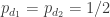 , which implies for instance that for (almost) any triangle with two sides in
  and the other side of unit length, exactly one of the first two sides is monochromatic. Presumably one can use this to create a contradiction.
Assuming this, then all we need to do is find a human proof of Marin's observation that at least five of the vertices have the same color as
  .
.
By the way, do we have algebraic expressions for the vertices ? Writing
  and
and  , I see that
  has magnitude
  and
and  has magnitude
  , so presumably the
  are multiples of
  by some powers of
  , and perhaps some other
  ?
?
The vertices and
and  are oriented directly upwards, so
  and
and  . The other vertices are simply rotations by
  in the appropriate direction, eg
  .
.
I don’t know offhand how to write these expressions entirely in terms of and
and  instead of
  . I will try to figure that out.
The vertex , which is pure imaginary and at distance
  from the origin, is
  .
.
The vertex , which is pure imaginary and at distance
  from the origin, is
  .
.
Boris, thanks for the explicit formulae!
I have now found a fairly simple proof of an improvement to the probability bound , namely that
  whenever
  . See Proposition 35 in http://michaelnielsen.org/polymath1/index.php?title=Probabilistic_formulation_of_Hadwiger-Nelson_problem . So the second part of my above proposal is now done; “all” that remains is to find a human proof that at least half of the vertices
  share the same color as
  .
.
Terry: that is very cool. I’m wondering whether the approach can be pushed further. (Of course any reduction from 1/2, however small, suffices for the purpose you are applying it to, but maybe a reduction below 23/47 would be useful for other purposes.) Intuitively it seems “wasteful” to switch from the hexagon to the pentagon without compensation. Can one infer anything from the fact that at least two of the 15 edges/diagonals of the hexagon BADFGE must be mono? It has seven edges of length d (the perimeter and DE) and the other eight all more than 1/2, so that’s more or less the same situation as the pentagon, but I’m just thinking that, well, 2/15 is more than 1/10…
Yes, it is certainly likely that the 1/92 term can be improved with more effort, particularly if one restricts the range of d a bit more to ensure that various distances stay above 1/2. In a hexagon it is guaranteed that there will be at least two monochromatic edges, not just one, so that may already lead to some gain.
A model problem would simply be to obtain the lower bound by a human proof. That is to say, suppose that one assumes that
  , thus all edges with length 1,
  , or
, or  are bichromatic. Can one get a contradiction? From Heule’s work (if I am reading it correctly) it seems that one can already do so in the group
  , using only the unit distances
  , the
, the  -distances
  , and the
  -distances
  . If one restricts to this group one gets an additional symmetry coming from the four-element Galois group of
  , in which one can conjugate
  while sending
  to
to  . In particular by using this symmetry one can always assume wlog that
  .
.
@Terry I just don’t get why your proof is so convoluted on the polymath blog. Isn’t it simpler to just take 6 isosceles triangles with sides, like ABC, ACD, just continue in the same way with ADE, AEF, AFG, AGH, and then conclude that ABDFH is monochromatic with probability ? From this, I think, one gets
  .
.
This should also work, though I don’t quite get the same numbers as you – for instance the probability for ABDFH monochromatic seems to be lower bounded by if I worked it out correctly. But one issue is that one needs all relevant distances to be at least 1/2 in order for Lemma 2 to be applicable, and this may place a more strict constraint on d if one uses your approach. Still I think it is worthwhile to try to optimise this argument. If for instance we can get
  below
below  then we only need to show that at least four out of ten vertices
  have the same color as
  , rather than five.
Yes, it is indeed . It comes from that there are
  edge of length
  , out of which we use
  in the final configuration. But I don’t think that the distance should be a problem, as instead of centering them around
  , we can keep on changing around which point we rotate, i.e., in the second step we can reflect
  to
to  . This way the minimal distance will be
  , just as in your original proof. And then the final calculation should give
  , thus
  . Oops, it seems that you made a mistake in polymath prop 35, as you need to multiply
  by
by  .
.
You’re right, the 94 should be a 188. On the other hand, by optimising your approach I can get the 188 (or 118) down to 62; see Proposition 36 on the wiki. I was in a hurry so I didn’t calculate the exact range of d for which the argument applies but this should just be some elementary trigonometry.
I’ve cleaned up the proof of Prop 36 (and also fixed some minor errors in Prop 35). If we suppose , then we have
 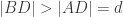 , thus it intuitively feels like we should be able to use some kind of induction on the length to get slightly better bounds. More precisely, if we define
  , then I think we win
  six times in the last equality of the proof and we can conclude
  , which gives
  . Is this correct?
This looks plausible, though I haven’t double checked the Euclidean geometry to make sure that all the lengths do indeed stay above so that one can iterate.
Philip wrote: “We now know that if we want a graph that cannot be 6-coloured it must have a radius greater than two.” Hm, yes – and indeed, we know that if we want a graph that cannot be 4-coloured it must have a radius greater than 0.869, and if we want a graph that cannot be 5-coloured it must have a radius greater than about 1.1 (see my sketches from yesterday). What’s the smallest-radius 5-chromatic graph we have so far? I think we must be quite close to 1. I wonder if we can use that.
I am trying to prefect some methods that I can use to eliminate cases for colouring a tiling. I think it may be useful to look at unit distance graphs, but instead of thinking about the colours at each vertex I look at colours around the vertex. Specifically I divide the neighbourhood around a vertex into sectors using lines perpendicular to edges that meet at the vertex and then consider colours in those sectors.
I want to be able to say that colours at different vertices can’t be monochromatic. E.g. in this diagram all the colours at f, e and d, must be different from all the colours at l, k and j, while the colours at a,b and c are different from g,h and i.
There may be more than one colour in a segment but I want to say that there is at least one colour in each sector such that the vertex is a limit point of points in the sector with that colour, and this exclusion condition holds.
What topological conditions must be imposed on the colouring for this to be true? I think it is true if tiled zones are used but is it more general?